Download
1 / 16
160 likes | 275 Views
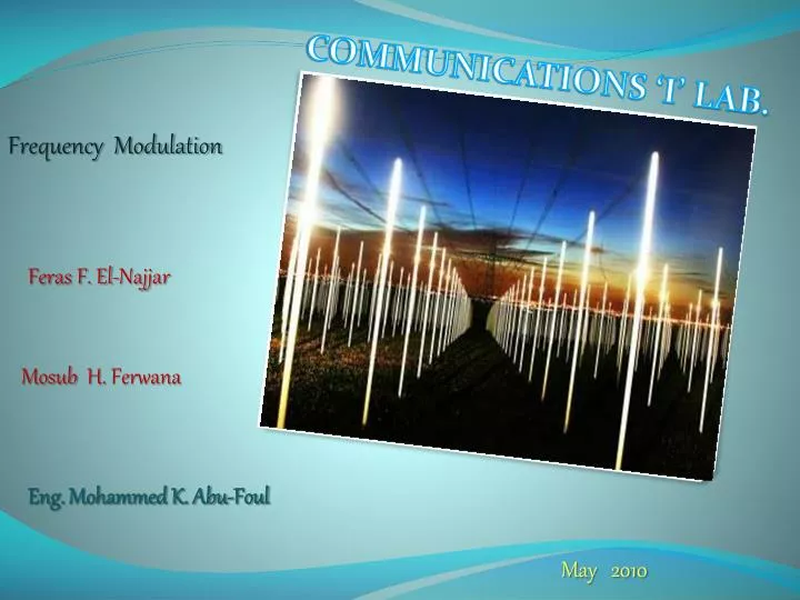
COMMUNICATIONS ‘I’ LAB. Frequency Modulation. Feras F. El- Najjar. Mosub H. Ferwana. Eng. Mohammed K. Abu-Foul. May 2010. Angle Modulation (Exponential Modulation )

E N D
COMMUNICATIONS ‘I’ LAB. Frequency Modulation Feras F. El-Najjar Mosub H. Ferwana Eng. Mohammed K. Abu-Foul May 2010
Angle Modulation (Exponential Modulation ) Is a techniques of modulation , where the angle of the carrier is varied in some manner with any modulating signal m(t) .
Phase Modulation (PM) Is one of two possible types of angle modulation , where the angle θ(t) is varied linearly with m(t) . θ(t)= ωc t + Kp * m(t) ψPM(t)= A cos [ ωc t + Kp * m(t)]
Frequency Modulation (FM) Is a form of modulation which represents information as variations in the instantaneous frequency of a carrier wave . ψFM(t)= A cos [ ωc t + Kf * ] Kf: constant sensitivity factor
The Instantaneous Frequency (ωi) ωi(max) = ωc + Kf * m(max) ωi(min) = ωc + Kf * m(min)
Frequency Deviation Frequency deviation rate is a result of message amplitude change . Kf : in radians Deviation Ratio (β) β = ∆f/B B.WFM = 2(∆f + B)
FM - Demodulation In FM Demodulation,the intelligence to be recovered is not in amplitude variations. it is in the variations of the instantaneous frequency of the carrier , either above or below the center frequency .
FM – Demodulation by direct differentiation In this method we differentiate the FM signal to get an AM signal, then we use an envelope detector.
MatLab Codes clear all fc=100; ts=1/(10*fc); fs=(1/ts); kf=80; wc=2*pi*fc; t=0:ts:2; m=sin(2*pi*t); y=cos(wc*t+(kf*2*pi*cumsum(m)).*ts); figure(1) subplot(211) plot(t,m) title('input signal') subplot(212) plot(t,y) title('fm modulation of input signal')
The code of magnitude spectrum of m(t) and the FM signal mf=fftshift(fft(m))*ts; delta=fs/length(mf); f=-fs/2:delta:fs/2-delta; figure(2) subplot(211) plot(f,abs(mf)) title('magnitude spectrum of input signal') a=fftshift(fft(y))*ts; delta=fs/length(a); f=-fs/2:delta:fs/2-delta; subplot(212) plot(f,abs(a)) title('magnitude spectrum of the fm')
The plot of the output signal after differentiator E=diff(y)/ts; figure(3) plot(E) title('the differentiation of fm ')
The plot of the output signal from the envelope detector vout(1)=E(1); t1=(0:length(E)-1)*ts; R=[10^5,10^4,10^3]*3.2; c=10^-6; for n=1:3 for i =2:length(E) if E(i)>vout(i-1) vout(i)=E(i); else vout(i)=vout(i-1).*exp(-ts/(R(n)*c)); end end figure(4) subplot(3,1,n) plot(t1,vout,t1,E) title(' the AM signal and envelope signal ') end
Thank You … And WeareReadyForany … Question !!!