Download
1 / 30
300 likes | 390 Views
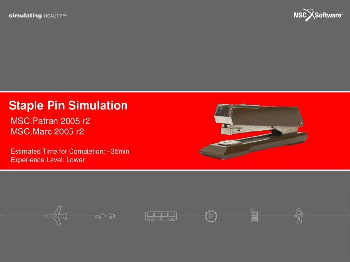
S taple P in S imulation. MSC.Patran 2005 r2 MSC.Marc 2005 r2. Estimated Time for Completion: ~35min Experience Level: Lower. Topics Covered. Topics covered in Modeling Defining the system of units. Importing Geometry file. Parasolid format (.x*t*)

E N D
Staple Pin Simulation MSC.Patran 2005 r2 MSC.Marc 2005 r2 Estimated Time for Completion: ~35min Experience Level: Lower
Topics Covered • Topics covered in Modeling • Defining the system of units. • Importing Geometry file. • Parasolid format (.x*t*) • Creating Surface by extruding curves. • Easiest way to create 3-D shell structure with uniform cross section. • Applying Equivalence. • It eliminates any duplicated nodes and cracks created by the mesher. • Creating Elastic-perfectly plastic material. • The material non-linearity is approximated by a constant. • Topic covered in Analysis • Applying Deformable and Rigid bodies contact. • Fixed and moved rigid bodies. • Applying Friction coefficient. • Applying Large Displacement/Large Strains Analysis. • Applying Load steps (Loading and Unloading). • Topics covered in Review • Creating XY plots and animations.
Problem Description Fmax=? b a • Rigid body motion and contact analysis are often used in break forming simulation. In this example, a staple pin is pushed by the upper rigid surface and formed due to the curvature of the lower rigid surface. • Loading: Upper rigid surface moves down to push a staple pin. • Unloading: Upper rigid surface goes back to its original position.
Problem Description • Given Parameters • System of Units • Length unit: mm • Mass unit: tonne • Time unit: sec • 1 force unit = tonne x mm/s^2 = 1N • 1 stress unit = N / mm^2 = 1e6 Pa • 1 density unit = tonne/mm^3 =1e-12 kg/m^3 • Aluminum pin • Dimensions: a=6, b=12, width=0.5, height=0.3 • Material properties: Young’s Modulus=63000, Poisson’s ratio=0.3, Yield strength=30, Density= 2.6989e-9 • Simplifying the problem • Apply Symmetric boundary conditions at the center of the pin. • ux=θy= θz=0 on the symmetric boundary. At lease ux=0 is required to obtain the desired solution. • Other possible simplifications. • Only half of the geometry can be used. • Instead Shell elements, use Beam elements.
Problem Description • Find the deformed shape of the staple pin and locate the maximum stress occurring. • Find the maximum load required.
Expected Results Loading Unloading • Von Mises Stress
Create Database and Import a Geometry File a d e f g h i j b c • Click File menu / Select New • In File Name enter staple.db • Click OK • Select Analysis Code to be MSC. Marc • Click OK • Click File menu / Select Import • Select Object to be Model • Select Source to be Parasolid xmt • Select the model file, stapler.xmt_txt • Click Apply. You will see the summary window for importing the Parasolid file. Click OK to close the window.
Create Surface a b c d e f g h Create Surfaces by extruding existing curves • Click Geometry icon • Select Action to be Create • Select Object to be Surface • Select Method to be Extrude • In Translation Vector, enter <0,0,0.5> • Uncheck Auto Execute • In Curve List, enter Curve 1:9 or select all lines in the view port • Click Apply
Create a Node a b c d e f g Create a node to control the upper rigid surface • Click Element icon • Select Action to be Create • Select Object to be Node • Select Method to be Edit • Uncheck Auto Execute • In Node Location List, enter [0,8.0,0] • Click Apply You can visualize nodes by toggling this icon.
Create Mesh Seed m l a b c d f g e i j k l m j k h Create bias mesh seeds on the existing curves. Two way bias • Click Element icon • Select Action to be Create • Select Object to be Mesh Seed • Select Type to be Two Way bias • In Number, enter 20 • In L2/L1, enter 4 • Uncheck Auto Execute • In Curve List, enter Curve 7 Surface 7.4 7.2 or select the top lines of the staple pin. • Click Apply One way bias Uniform mesh Repeat (d) – (i) for the following new sets of Mesh Seeds
Create Mesh and Apply Equivalence a b c d e f g h i • Select Action to be Create • Select Object to be Mesh • Select Type to be Surface • In Surface List, enter Surface 1 2 6:8 or select all surfaces of the pin • Click Apply • Select Action to be Equivalence • Select Object to be All • Select Method to be Tolerance Cube • Click Apply Applying Equivalence shows the eliminated nodes on the veiwport This will eliminate any extra overlapping nodes created by the mesher. See below for the comparison.
Create the Material Properties q a b c d e f g h i j k l m n o p r • Click Materials icon • Select Action to be Create • Select Object to be Isotropic • Select Method to be Manual Input • In Material Name, enter Aluminum • Click Input Properties • Select Constitutive Model to be Elastic • In Elastic Modulus, enter 63000 • In Possion Ratio, enter 0.3 • In Density, enter 2.6989e-9 • Click OK • Click Apply • Click Input Properties again • Select Constitutive Model to be Plastic • Select Type to be Perfectly Plastic • In Yield Stress, enter 30 • Click OK • Click Apply
Create the Element Properties a b c d e f g h i j k l m n • Click Properties icon • Select Action to be Create • Select Object to be 2D • Select Type to be Thick Shell • In Property Set Name, enter pin • Select Options to beHomogeneous andStandard Formulation • Click Input Properties • Click Mat Prop Name icon • Select Aluminum • In [Thickness], enter 0.3 • Click OK • In Application Region, enter Surface 1 2 6:8 or select elements on the pin using the mouse left button • Click Add • Click Apply
Create Boundary Conditions e a b c d o g f i j k l m n h Create the Boundary Conditions for driving on and off of the top rigid body. • Click Loads/BCs icon • Select Action to be Create • Select Object to be Displacement • Select Type to be Nodal • In New Set Name, enter drive_on • Click Input Data • In Translations, enter <0,-6.5,0> • In Rotations, enter <0,0,0> • Click OK • Click Select Application Region • Select Geometry Filter to be FEM • In Select Nodes, enter Node 1 or select the nodes made above the rigid body • Click Add • Click OK • Click Apply Drive on/off Repeat (e) – (o) for the following new sets of BCs Sym_disp
Create Boundary Conditions a b c d e f g h i j k l Create the Deformable Contact Body. • Select Action to be Create • Select Object to be Contact • Select Type to be Element Uniform • Select Option to be Deformable Body • In New Set Name, enter contact_mid • Select Target Element Type to be 2D • Click Select Application Region • Select Geometry Filter to be Geometry • In Select Nodes, enter Surface 1 2 6:8 or select all surfaces of the pin • Click Add • Click OK • Click Apply
Create Boundary Conditions p o a b c d e f h i j k l m n g Create the Rigid Contact Bodies. • Select Action to be Create • Select Object to be Contact • Select Type to be Element Uniform • Select Option to be Rigid Body • In New Set Name, enter contact_top • Select Target Element Type to be 2D • Click Input Data • Select Motion Control to be Force/Moment • In First Control Node, enter Node 1, or select the controlling node. • Click OK • Click Select Application Region • Select Geometry Filter to be Geometry • In Select Nodes, enter Surface 9 or select the rigid body above the pin • Click Add • Click OK • Click Apply Repeat (e) – (p) for the following new sets of BCs
Create Boundary Conditions a b c d e f g h i j Correct the Contact Normals for the rigid bodies. The Contact Normals of the top surface need to be flipped. • Select Action to be Modify • Select Object to be Contact • Select Type to be Element Uniform • Select Option to be Rigid Body • In Select Set to Modify, enter contact_top • Select Target Element Type to be 2D • Click Modify Data • Click OK • Click Apply
Create Boundary Conditions n m a b c d e g h i j k l f Create the Fixed Boundary Conditions • Select Action to be Create • Select Object to be Inertial Load • Select Type to be Element Uniform • In New Set Name, enter gravity • Select Target Element Type to be 2D • Click Input Data • In Trans Accel, enter <0,-9810,0> • Click OK • Click Select Application Region • Select Geometry Filter to be Geometry • In Select Nodes, enter Surface 1 2 6:8 or select the Surfaces of the pin • Click Add • Click OK • Click Apply You must see all Boundary Conditions as shown in this figure
Create Load Cases a b c d e f g Create the Loading and Unloading load cases • Click Load Cases icon • Select Action to be Create • In Load Case Name, enter loading • Click Input Data • In Select Individual Loads/BCs, selectConta_contact_bottomConta_contact_midConta_contact_topDispl_drive_onDispl_sym_disp • Click OK • Click Apply Repeat (c) – (g) for the following sets of BCs You must see the assigned Load/BCs in this window after selecting the individual Loads/BCs
Run Analysis q p a b c d e f g h i j k l m n o Analysis Options for the first load step • Click Analysis icon • Select Action to be Analyze • Select Object to be Entire Model • Select Method to be Full Run • In Job Name, enter staplePin • Click Load Step Creation • In Load Step Name, enter LoadingStep • Click Select Load Cases • In Available Load Cases, select loading • Click OK • Click Solution Parameters • Select Linearity to be NonLinear • Select Nonlinear Geometry Effects to be Large Displacement/Large Strains • Click Load Increment Parameters • Select Increment Type to be Adaptive • In [Trial Time Step Size:], enter 0.05 • Click OK
Run Analysis a b c d e f g h Analysis Options for the first and the second load steps • Click Iteration Parameters • In Max # of Iterations per Increment, enter 20 • Click OK • Click Contact Table • Click Touch All • Click OK • Click OK • Click Apply Repeat from (g) in the previous slide to (h) in this slide for the Second Load Step
Run Analysis and Monitor a b c d e f g h Select Load Steps to run and Run Analysis • Click Load Step Selection • In Existing Load Steps, select LoadingStepUnloadingStep • In Selected Load Steps, select Default Static Step • Click OK • Click Apply • Select Action to be Monitor • Select Object to be Job • Click Apply You must see the Load Steps in a certain order you want to run.
Read Results a b c d e f g h i Read Results File • In the Marc Job Monitoring window, if the Exit Number is 3004, the problem has been solved successfully. • Click Cancel • Select Action to be Read Results • Select Object to be Result Entities • Select Method to be Attach • Click Select Results File • Select staplePin.t16 • Click OK • Click Apply
Reviewing the Results h i j k a b c d e f g Review the Displacement Results and Stress Results • Click Results icon • Select Action to be Create • Select Object to be Quick Plot • In Select Result Cases, select the last results Time=1.0 is the end of the first load stepTime=2.0 is the end of the first load step • In Select Fringe Result, select Displacement, Translation • In Select Deformation Result, select Displacement, Translation • Click ApplyCheck the viewport to see the result plot • In Select Fringe Result, select Stress, Global System • Select Quantity to be von Mises • In Select Deformation Result, select Displacement, Translation • Click ApplyCheck the viewport to see the result plot
Reviewing the Results a b c d e f g h i Review the Reaction force at the bottom • Select Action to be Create • Select Object to be Graph • Select Method to be Y vs X • In Select Result Cases, select all results Time=1.0 is the end of the first load stepTime=2.0 is the end of the first load step • Select Y: to be Global Variable • Select Variable: to be Body contact_bottom, Force Y • Select X: to be Global Variable • Select Variable: to be Time • Click ApplyCheck the viewport in new window to see the result graph
Results • Rigid body displacement
Results • Load requirement for step 1 • Total reaction force (Ry) at the bottom surface = - load requirement FMax = 0.28N RMin = -0.28N
Results • Von Mises stress at the end of load step 1 σMax=32.1e6 Pa • at the end of load step 2 σMax=24.6e6 Pa
Further Analysis (Optional) • Problem modification • Instead Aluminum, use Steel as a pin. Find the load requirement. • Material properties of Steel: Young’s Modulus=2.1e5MPa, Poisson’s ratio=0.3, Yield strength=250MPa • What do you expect if you staple 10 sheets(1mm) of paper together? Will the required load be increased or decreased? • Modeling • If you want to use ‘cm’ as your length unit, what other units do you need to change? • Try without the gravity in the load step 2. • Can you find the symmetrical results without the symmetric condition at the center of the pin? • Solution options • Increase [Trial Time Step Size:]for the load step 2. What value is the maximum to obtain the result?