Download
1 / 16
160 likes | 354 Views
Piet Martens Montana State University, Bozeman, MT, USA & Paul Wood University of St Andrews, Fife, Scotland. FLUX CANCELLATION IN PROMINENCE FORMATION. BACKGROUND. Undergraduate summer project Study of 3 different prominences Used H-alpha, MDI, EIT data

E N D
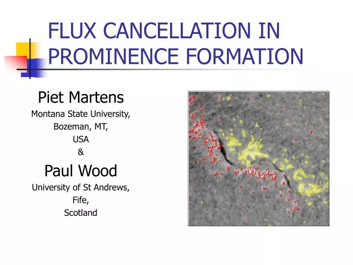
Piet Martens Montana State University, Bozeman, MT, USA & Paul Wood University of St Andrews, Fife, Scotland FLUX CANCELLATION IN PROMINENCE FORMATION
BACKGROUND • Undergraduate summer project • Study of 3 different prominences • Used H-alpha, MDI, EIT data • Look for evidence of flux cancellation during filament formation • Web-site: solar.physics.montana.edu/wood
PROMINENCES STUDIED The 3 prominences I studied in Montana, clockwise from the top: August 1997, September 1997 & June 1999.
FLUX CANCELLATION PAPER • September 1997 prominence • Identify all flux cancellation • Calculate approx. flux change • Relate to change in filament morphology • Compare with theoretical models
PROMINENCE DATA (1) Active Region Map, 31 August 1997. Prominence forms between 3 decaying active regions
PROMINENCE DATA (2) EIT image with MDI overlay. Note the lack of connections across the PIL, consistent with the presence of a filament channel.
PROMINENCE DATA (3) H-alpha pictures, taken from Meudon Observatory, Paris, 25 Sept 08:02, and Big Bear Solar Observatory, 27 Sept 16:14
THE MAGNETIC FIELD (1) H-alpha image with magnetic field contours over-laid. Contour levels = 40, 60, 80, 100 G White = positive flux Black = negative flux
THE MAGNETIC FIELD (2) The magnetic field at the photosphere below the filament. Circles 1-5 show the areas where flux cancellation was seen to occur.
PROJECTED IMAGE Example of a projected magnetogram image. Each pixel now represents the same area on the sun.
RESULTS Magnetic Flux changes calculated for each area. Undetermined areas are those where individual flux patches could not be isolated.
FLUX IN PROMINENCE Measured radius of filament ~ 10,000 km. Axial field in quiescent prominence ~ 10 G (Leroy et al.), hence flux ~ 3 x 10^19 Mx, of the order of amounts cancelled, and much less than unsigned flux in either decaying AR.
FLUX EMERGENCE Circles 1 and 2 show sites where positive flux has emerged in areas of predominantly negative field. The table shows the change in positive flux over time for the 2 areas.
LINKAGE MODEL Observations support "linkage" (Martens & Zwaan 2001) but not emergence of loop (e.g. Rust), or cancellation in pre-existing arcade (van Ballegooijen & Martens)
COMPARISONS • Chae et al, Solar Physics, 2002 • Study cancellation for 2 cases, using MDI • Flux levels 3 x 10¹⁸ Mx per hour. • Litvinenko & Martin, Solar Physics, 1999 • Look at cancellation at end of a filament channel. • Cancellation rate 1019 Mx per hour.
KEY POINTS • Flux cancellation seen at bends and each end of forming prominence. • Change in flux 1019 Mx, similar to flux in prominence body. • Observations support head-to-tail linkage models. • These are merely 4 examples in the formation of a single prominence!