Download

1 / 12
120 likes | 252 Views
Cancellation of magnetic flux in magnetograms has been defined in observational terms as "the mutual apparent loss of magnetic flux in closely spaced features of opposite polarity."

E N D
Cancellation of magnetic flux in magnetograms has been defined in observational terms as "the mutual apparent loss of magnetic flux in closely spaced features of opposite polarity." Physically, this removal of flux could correspond to one of three mechanisms: (i) the emergence of U-shaped magnetic loops, (ii) the submergence of Omega-shaped loops, or (iii) reconnection in the magnetogram layer. Evidence has been reported for all three of these mechanisms, but does one predominate? We can investigate cancellation mechanisms at work in an active region's magnetic fields using time-averaged Doppler shifts along polarity inversion lines (PILs) of the line-of-sight (LOS) magnetic field near disk center. Along these PILs, the LOS component of the magnetic field vanishes, so LOS flows inferred from Doppler shifts are perpendicular to the magnetic field. If the evolution is ideal, such flows imply the transport of magnetic flux across the atmospheric layer imaged in the magnetogram. As a preliminary step in our study, we present an innovative method to remove biases in the measured Doppler velocities due to offset in the line-center position, which might arise from a well-known correlation between brightness and blueshifts in the convecting photospheric plasma Using HMI to Understand Flux Cancellation by Brian Welsch1, George Fisher1, Yan Li1, and Xudong Sun2 1Space Sciences Lab, UC-Berkeley,2Stanford University
Q: How is flux removed from the photosphere? • Each 11-year cycle, c. 3000 active regions, each with c. 1022Mx, emerge. • What processes remove all this flux? • The short answer is CANCELLATION --- the “mutual apparent loss of flux in closely spaced magnetogram features of opposite polarity” (Livi et al. 1985)
Q: But what is cancellation? Cancellation could be any of three processes: • Doppler shifts on PILs can distinguish between these!
Q: Which process predominates in active regions? Which model more accurately describes the Sun?
Changes in LOS flux are quantitatively related to PIL Doppler shifts multiplied by transverse field strengths. From LOS m’gram: (Eqn. 1) From Faraday’s law, Since flux can only emerge or submerge at a PIL, (Eqn. 2) Summed Dopplergram and transverse field along PIL pixels. • Inthe absence of errors, ΔΦLOS/Δt =ΔΦPIL/Δt.
Let’s test the method with HMI data! An automated method (Welsch & Li 2008) identified PILs in a subregion of AR 11117. Note predominance of redshifts.
Problem: We must remove the convective blueshift! HMI’s Doppler shifts are not absolutely calibrated! (Helioseismology uses time differences in Doppler shifts.) There’s a well-known intensity-blueshift correlation, because rising plasma (which is hotter) is brighter (see, e.g., Gray 2009; Hamilton and Lester 1999; or talk to P. Scherrer). Because magnetic fields suppress convection, lines are redshifted in magnetized regions. From Gray (2009): Bisectors for 13 spectral lines on the Sun are shown on an absolute velocity scale. The dots indicate the lowest point on the bisectors. (The dashed bisector is for λ6256.) Lines formed deeper in the atmosphere, where convective upflows are present, are blue-shifted.
So we must calibrate the bias in the zero-velocity v0 in estimated Doppler shifts before we can study cancellation. From Eqn. 2, a bias velocity v0 implies := “magnetic length” of PIL • ButΔΦLOSshould match ΔΦPIL, so we can solve for v0: (Eqn. 3) NB: v0 should be the SAME for ALLPILs==> solve statistically!
We have solved for v0 using data from > 100 PILs in three successive magnetogram triplets from Fig. 3. Incorporating error bars on estimates of ΔΦ’s is still a work in progress; ideally, we’d estimate v0 using total least squares.
The inferred offset velocity v0 can be used to correct Doppler shifts along PILs.
Conclusions • We have demonstrated a method to correct the bias velocity v0 in HMI’s Doppler velocities from convective-blueshifts. • Using v0-corrected Doppler data, we can study flux cancellation in active regions, to determine which physical process underlies cancellation.
Future Work • Incorporate error bars on estimates of ΔΦ’s and magnetic lengths, and investigate estimation of v0 via total least squares. • Errors are present in both magnetic lengths and ΔΦ’s. • Actually investigate cancellation! • Investigate statistics of cancellation mechanisms in both active regions (and quiet sun). • Extrapolate flux submergence rates over solar cycle (and quiet Sun flux turnover time) to constrain flux recycling in solar cycle (and quiet sun) dynamo.