Download
1 / 21
210 likes | 314 Views
MHD Simulations of Flux Cancellation on the Sun*. Judy Karpen, Spiro Antiochos, Rick DeVore, and Mark Linton. *Work supported by ONR and NASA. Outline. What is flux cancellation? Origins Methodology Results Conclusions Questions. What is Flux Cancellation?.

E N D
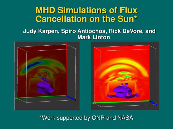
MHD Simulations of Flux Cancellation on the Sun* Judy Karpen, Spiro Antiochos, Rick DeVore, and Mark Linton *Work supported by ONR and NASA
Outline • What is flux cancellation? • Origins • Methodology • Results • Conclusions • Questions
What is Flux Cancellation? • Observational definition: the disappearance of the line-of-sight component of magnetic flux where opposite polarities meet. • Each magnetogram measures the field at 1 height (photosphere or chromosphere); rarely obtained at 2 or more heights at the same time (e.g., Harvey et al. 1993). Time series of magnetograms showing the magnetic flux changes (crosses show explosive event locations). The tick interval is 5” (3600 km). The brighter features are positive (north) polarity magnetic fluxes, and the darker features are negative (south) polarity fluxes. The positive magnetic flux indicated by the arrow is decreasing with time. [images from BBSO]
Possible Origins of Flux Cancellation • emergence of concave-upward flux (U loops) • Can result from reconnection below the photosphere/ chromosphere, but only the shallowest U loops can overcome mass loading • submergence of concave-downward flux (Omega loops) • If due to reconnection above the photosphere/ chromosphere, then the lower (concave-downward) region of newly reconnected flux must submerge completely below the magnetogram level. • Magnetic reconnection in the photosphere/ chromosphere itself • unlikely to occur only in those few layers observed by magnetographs). Role of reconnection assumed but not well tested
Cancellation and Filament Channel Formation Van Ballegooijen & Martens (1989) Problem: do required surface flows exist?
Flux Emergence and Sheared Arcades • Strongly sheared flux rope is mainly trapped by mass loading. What emerges forms a sheared arcade, but shear is not concentrated enough at PIL (Magara et al. 2007). • Weakly sheared flux rope emerges more, but shear is weaker than observed (Magara 2006). Can flux cancellation concentrate magnetic shear at the PIL in our sheared 3D arcade model?
Methodology • 3D MHD simulations with ARMS*: • Finite-difference FCT • Cartesian geometry • Adaptive mesh refinement with PARAMESH • Numerical resistivity • No radiation, heating, or thermal conduction • Visualization with HelioSpace* *developed, tested, and used extensively under DoD CHSSI and HPCM programs, and NASA’s HPCC
Initial Conditions • Magnetic Field: Lundquist flux tube embedded in potential arcade • 1.5 < |B|max < 600 G • Plasma: hydrostatic equilibrium atmos- phere, -1.8 < log8 • Closed boundaries Fieldlines and plasma System size: 20 Mm x 20 Mm x 10 Mm (symmetry in z)
Imposed Subphotospheric Flow • Subsurface Flow: two-cell convection-like pattern below photosphere (1), converging at polarity inversion line • max. Vy = +2.3 km s-1 max. Vx = -6.0 km s-1 • Cosine fall-off in z so Vx and Vy = 0 at zmax Streamlines and |B|
Global Properties • Break in KE at 1000s because subsurface flow was ramped up from 0 to 1000 s, held steady thereafter
Early development (t=1000-2000 s) jz |B| |v|
Plasmoid formation (t=1000-2000 s) log 1000 s 1200 s 1400 s 1600 s 1800 s 2000 s
Asymmetry develops (t=2500-3000 s) 2500 s 2600 s 2600 s |j| 2600 s 2800 s
Late Development (t=3000-5000 s) jz |v| jz |B|=300 G
Magnetograms 100 s 2000 s 3000 s 4000 s 5000 s 6000 s |Bx| < 100 G; height = -2.5 Mm (photosphere)
Preliminary Conclusions • Subsurface flows acting on unsheared flux can produce reconnection and magnetographic signatures of cancellation at photosphere • Cancellation of unsheared flux yields complex magnetic structure both below the photosphere and in the corona above • Classical signature of reconnection (jets) does not occur, perhaps due to strong downflows • Need better resolution -- turn adaptivity on
Adaptive Gridding Initial grid: 3 levels, magenta is finest
Adaptive Gridding t=1000 s: 4 levels, magenta is finest
Adaptive Gridding t=2000 s: 4 levels, magenta is finest
Questions • Any plasmoids (flux ropes) fully in corona? • No reconnection jets? • Source of periodic structure in z? • How much flux cancels at the photosphere? • What happens when sheared flux is cancelled? Tune in next time….