Download
1 / 19
190 likes | 344 Views
Verifying fossil fuel CO 2 emissions with CMAQ. Zhen Liu , Cosmin Safta , Khachik Sargsyan , Bart G. van Bloemen Waanders , Ray P. Bambha , Hope A. Michelsen Sandia National Laboratories, CA/NM Tao Zeng Georgia Department of Natural Resources, GA CMAS 2012 15 October 2012.

E N D
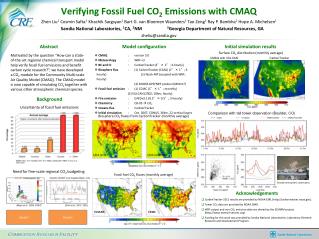
Verifying fossil fuel CO2 emissions with CMAQ Zhen Liu, CosminSafta, KhachikSargsyan, Bart G. van BloemenWaanders, Ray P. Bambha, Hope A. Michelsen Sandia National Laboratories, CA/NM Tao Zeng Georgia Department of Natural Resources, GA CMAS 2012 15 October 2012
Atmospheric CO2 trend and carbon cycle NRC, 2010: Verifying Greenhouse Gas Emissions: Methods to Support International Climate Agreements, pp16, Fig. 1.3 http://www.esrl.noaa.gov/gmd/ccgg/trends/ Growing fossil fuel CO2 emission Rising atmospheric CO2 concentrations
Uncertainty of Fossil Fuel CO2 emissions Annual average ? ? (higher uncertainty after temporal allocation) gridded Global: NRC, 2010. Country: EPA, 2012. State, county and 1-10km: Gurney et al., 2009, ES&T Verifying fossil CO2emissions is “firmly on the agenda of science, politics, and business”. [Marland, 2008, J. Ind. Ecol., 136–139]
Verifying Fossil Fuel CO2 Emissions “A signal-to-noise problem” Satellite GOSAT (Los Angeles Basin, CA) Aircraft (Indianapolis, IN) 3.2±1.5 ppm [Mays et al., 2009, ES&T] [Kortet al., 2012, GRL] Model? Model? Can a state-of-the-art CTM help verify fossil fuel CO2 emissions?
3-D Eulerian Regional CO2 Modelingusing CMAQ • Add a CO2 module in CMAQ • Widely used and well tested CTM, large user community; • Highly modularized codes makes adding species/processes easy; • Adaptable nested model domains enables high resolution modeling. • Goals: • Quantitatively examine model skills/errors on different time/spatial scales; • Develop model diagnostics and inverse modeling approach to pinpoint fossil fuel emissions; • Construct regional CO2 budget and quantify its uncertainties.
Configuration of the CMAQ CO2 module (done/under development) • CMAQ :version 5.0 • Meteorology: WRF • BC/IC :CarbonTracker (CT) (3°× 2°; 3-hourly) • Biosphere flux : (1) CarbonTracker (CASA) (1°× 1°) (2) VPRM (3) Sib3 • Fossil fuel emission :(1) CDIAC (1°× 1°; monthly) • (2) VULCAN (2002; 10km; hourly) • Fire emission:GFEDv3.1 (0.5°× 0.5°; 3-hourly) • Chemistry :CB-05 CO2 • Oceans flux:CarbonTracker • Benchmark: Oct. 2007, U.S. 36km, 22L
Benchmark simulation results (30m above ground) with CDIAC (1°× 1°, annual average) fossil fuel emission inventory CMAQ-CDIAC CarbonTracker • Root Mean Square Deviation (RMSD) = 0.47 ppm
Benchmark simulation results (30m above ground) with VULCAN(10km, hourly) fossil fuel emission inventory CMAQ-VULCAN CarbonTracker • Root Mean Square Deviation (RMSD) = 0.48 ppm
Benchmark simulation results (0-1500m average) with VULCAN (0.1°× 0.1°, hourly) fossil fuel emission inventory CMAQ-VULCAN CarbonTracker • Some hotspots could still be seen (> 4ppm enhancement) • Root Mean Square Deviation (RMSD) = 0.43 ppm
Model Evaluation: Boulder Atmospheric Observatory 40mile north of Denver; elev. 1584 masl; 300m above ground http://www.esrl.noaa.gov/gmd/ccgg/towers/#bao
Summary and Future Plan • Findings • Transport difference between CMAQ (36km) and TM5 (1°× 1°) only leads to 0.47 ppm Root Mean Square Deviation (RMSD) near the surface in terms of monthly mean CO2 distribution. • 36km CMAQ with hourly VULCAN (10km) emission inventory is capable of capturing urban CO2 hotspots in the contiguous U.S. and diurnal pattern of CO2 downwind of urban Denver. • Some hotspots might be observed using the PBL column average metric. • To-dos • Implementing finer resolution biosphere module (VPRM) and transport; • Adding secondary CO2 source (oxidation of CO and VOCs) in CMAQ; • Comprehensive model evaluation with tower and aircraft data.
Acknowledgement • CarbonTracker-2011 results are provided by NOAA ESRL (http://carbontracker.noaa.gov). • Tower CO2 data are provided by NOAA GMD. • WRF output and non-CO2 emission data are shared by the SESARM project (http://www.metro4-sesarm.org). • Funding for this work was provided by Sandia National Laboratories, Laboratory Directed Research And Development Program.
Benchmark simulation resultswith VULCAN (0.1°× 0.1°, hourly) fossil fuel emission inventory CMAQ-VULCAN CarbonTracker (500m above ground)
CarbonTracker (CT2011) http://www.esrl.noaa.gov/gmd/ccgg/carbontracker/ [Peters et al., 2007, PNAS] Meteorology : ECMWF (1°× 1° nested over NA) Biosphere : Carnegie-Ames-Stanford-Approach (CASA) Ocean :[Jacobson et al., 2007] Fossil fuel : CDIAC [Oda and Maksyutov, 2011] Fire : GFEDv3.1 Observations : NOAA ESRL, CSIRO, IPEN-CQMA