Download
1 / 1
10 likes | 114 Views
A multiresolution random field model for estimating fossil-fuel CO 2 emissions.

E N D
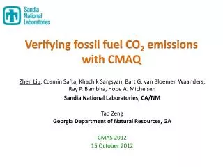
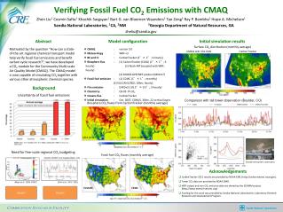
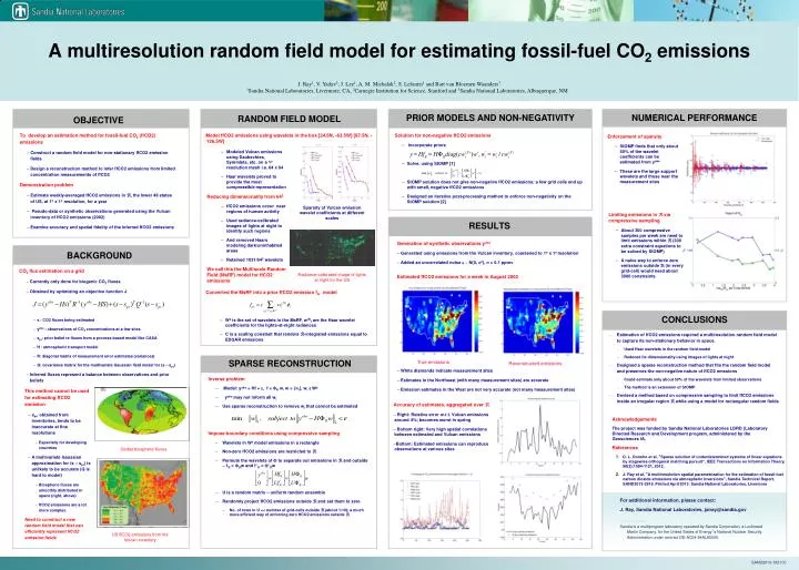
A multiresolution random field model for estimating fossil-fuel CO2 emissions J. Ray1, V. Yadav2, J. Lee1, A. M. Michalak2, S. Lefantzi1 and Bart van Bloemen Waanders31Sandia National Laboratories, Livermore, CA, 2Carnegie Institution for Science, Stanford and 3Sandia National Laboratories, Albuquerque, NM PRIOR MODELS AND NON-NEGATIVITY NUMERICAL PERFORMANCE • RANDOM FIELD MODEL • Model ffCO2 emissions using wavelets in the box [24.5N, -63.5W] [87.5N, -126.5W] • Solution for non-negative ffCO2 emissions • Incorporate priors • Solve, using StOMP [1] • StOMP solution does not give non-negative ffCO2 emissions; a few grid cells end up with small, negative ffCO2 emissions • Designed an iterative post-processing method to enforce non-negativity on the StOMP solution [2] OBJECTIVE To develop an estimation method for fossil-fuel CO2 (ffCO2) emissions • Construct a random field model for non-stationary ffCO2 emission fields • Design a reconstruction method to infer ffCO2 emissions from limited concentration measurements of ffCO2 Demonstration problem • Estimate weekly-averaged ffCO2 emissions in R, the lower 48 states of US, at 1o x 1o resolution, for a year • Pseudo-data or synthetic observations generated using the Vulcan inventory of ffCO2 emissions (2002) • Examine accuracy and spatial fidelity of the inferred ffCO2 emissions Accuracy of estimates, aggregated over R • Right: Relative error w.r.t. Vulcan emissions around 4%; becomes worst in spring • Bottom right: Very high spatial correlations between estimated and Vulcan emissions • Bottom: Estimated emissions can reproduce observations at various sites RESULTS Estimated ffCO2 emissions for a week in August 2002 • White diamonds indicate measurement sites • Estimates in the Northeast (with many measurement sites) are accurate • Emission estimates in the West are not very accurate (not many measurement sites) Generation of synthetic observations yobs • Generated using emissions from the Vulcan inventory, coarsened to 1o x 1o resolution • Added an uncorrelated noise e ~ N(0, s2), s = 0.1 ppmv • Enforcement of sparsity • StOMP finds that only about 50% of the wavelet coefficients can be estimated from yobs • These are the large support wavelets and those near the measurement sites • Modeled Vulcan emissions using Daubechies, Symmlets, etc. on a 1o resolution mesh i.e. 64 x 64 • Haar wavelets proved to provide the most compressible representation • Reducing dimensionality from 642 • ffCO2 emissions occur near regions of human activity • Used radiance-calibrated images of lights at night to identify such regions • And removed Haars modeling dark/uninhabited areas • Retained 1031/642 wavelets • We call this the Multiscale Random Field (MsRF) model for ffCO2 emissions Sparsity of Vulcan emission wavelet coefficients at different scales • Limiting emissions in R via compressive sampling • About 300 compressive samples per week are need to limit emissions within R (300 extra constraint equations to be solved by StOMP) • A naïve way to enforce zero emissions outside R (in every grid-cell) would need about 3000 constraints • BACKGROUND • CO2 flux estimation on a grid • Currently only done for biogenic CO2 fluxes • Obtained by optimizing an objective function J • s : CO2 fluxes being estimated • yobs : observations of CO2 concentrations at a few sites • spr: prior belief re fluxes from a process-based model like CASA • H : atmospheric transport model • R: diagonal matrix of measurement error estimates (variances) • Q: covariance matrix for the multivariate Gaussian field model for (s – spr) • Inferred fluxes represent a balance between observations and prior beliefs Radiance-calibrated image of lights at night for the US • Converted the MsRF into a prior ffCO2 emission fpr model • Ws is the set of wavelets in the MsRF, w(X)I are the Haar wavelet coefficients for the lights-at-night radiances • C is a scaling constant that renders R-integrated emissions equal to EDGAR emissions • CONCLUSIONS • Estimation of ffCO2 emissions required a multiresolution random field model to capture its non-stationary behavior in space. • Used Haar wavelets in the random field model • Reduced its dimensionality using images of lights at night • Designed a sparse reconstruction method that fits the random field model and preserves the non-negative nature of ffCO2 emssions • Could estimate only about 50% of the wavelets from limited observations • The method is an extension of StOMP • Devised a method based on compressive sampling to limit ffCO2 emissions inside an irregular region R while using a model for rectangular random fields SPARSE RECONSTRUCTION True emissions Reconstructed emissions • Inverse problem • Model: yobs = Hf + e, f = FR w, w = {wi}, wi ε Ws • yobs may not inform all wi • Use sparse reconstruction to remove wi that cannot be estimated • Impose boundary conditions using compressive sampling • Wavelets in Ws model emissions in a rectangle • Non-zero ffCO2 emissions are restricted to R • Permute the wavelets of F to separate out emissions in R and outside – fR = FRw and f’R = F’Rw • U is a random matrix – uniform random ensemble • Randomly project ffCO2 emissions outside R and set them to zero • No. of rows in U << number of grid-cells outside R (about 1/10); a much more efficient way of enforcing zero ffCO2 emissions outside R • This method cannot be used for estimating ffCO2 emission • spr, obtained from inventories, tends to be inaccurate at fine resolutions • Especially for developing countries • A multivariate Gaussian approximation for (s – spr) is unlikely to be accurate (Q is hard to model) • Biospheric fluxes are smoothly distributed in space (right, above) • ffCO2 emissions are a lot more complex. • Need to construct a new random field model that can efficiently represent ffCO2 emission fields Acknowledgements The project was funded by Sandia National Laboratories LDRD (Laboratory Directed Research and Development program, administered by the Geosciences IA. • References • D. L. Donoho et al, “Sparse solution of underdetermined systems of linear equations by stagewise orthogonal matching pursuit”, IEEE Transactions on Information Theory, 58(2):1094-1121, 2012. • J. Ray et al, “A multiresolution spatial parametrization for the estimation of fossil-fuel carbon dioxide emissions via atmospheric inversions", Sandia Technical Report, SAND2013-2919. Printed April 2013. Sandia National Laboratories, Livermore Global biospheric fluxes For additional information, please contact: J. Ray, Sandia National Laboratories, jairay@sandia.gov • • • • • • • • • • • • • • • Sandia is a multiprogram laboratory operated by Sandia Corporation, a Lockheed Martin Company, for the United States of Energy’s National Nuclear Security Administration under contract DE-AC04-94AL85000. US ffCO2 emissions from the Vulcan inventory SAND2013-10211C