Download
1 / 57
590 likes | 690 Views
Solid-state NMR Training Course. Making a measurement. Routine set up of a CPMAS measurement. Assumptions:. Spin-½ nuclei. A standard sample (with known behaviour) is available. glycine. adamantane. CaHPO 4 ·2H 2 O. tetrakis ( trimethylsilyl ) silane (TTMSS). hexamethylbenzene (HMB).

E N D
Solid-state NMR Training Course Making a measurement
Routine set up of a CPMAS measurement Assumptions: Spin-½ nuclei A standard sample (with known behaviour) is available glycine adamantane CaHPO4·2H2O tetrakis(trimethylsilyl)silane (TTMSS) hexamethylbenzene (HMB) brushite The spectrometer is operating correctly and is in a state such that only fine tuning (checking/calibration) is required
The magic-angle Method 1 – 79Br, maximising the rotary echoes/sidebands from KBr Advantages: 79Br resonance is close to 13C (@9.4 T 100.25 MHz vs. 100.56 for 13C) No decoupling required Shimming not critical Good after repair or maintenance when angle badly set
The magic-angle Method 1 – maximising the rotary echoes/sidebands from KBr FID (Free Induction Decay) rotary echo (separation = rotor period) Acquire Adjust time / ms centreband on resonance
The magic-angle Method 1 – maximising the rotary echoes/sidebands from KBr time / ms Acquire – adjust – acquire …….
The magic-angle (Acquire)n – adjust – (acquire)n ….. gives more precision n = 64 @ 0.2 s, 45o pulse @ 4 kHz (maybe a problem) Good for most samples … … unless they contain highly anisotropic environments (>C=O, C-D, >M-)
Excitation methods optional Direct excitation: Pulse on X, observe on X Cross polarisation:
Cross polarisation Usually 1H to nX 1H Transfer of magnetisation (polarisation) nX
Cross polarisation vs. direct excitation Almost all measurements are …. pulse(s) – acquire – wait – pulse(s) – acquire – wait ….. DE RD RD recycle delay recycle pulse delay d1 RD depends on T1X
Spin-lattice relaxation T1 : Spin-lattice relaxation time constant Equilibrium magnetisation at time t after excitation (which will contribute to the signal after the next excitation) T1 : ultimately depends on molecular motion and is different (in principle) for each nuclide and each type of environment
Cross polarisation vs. direct excitation DE RD RD depends on T1X
Cross polarisation vs. direct excitation DE Repetition rate depends on T1X CP Repetition rate depends on T1H
Cross polarisation vs. direct excitation T1H : a single, molecule-wide average is measured 1.7 s T1C : different for each carbon. Average value (excluding CH3) 190 s. T1C (CH3) is approximately 1 s.
Cross polarisation vs. direct excitation Another advantage for CP over DE: For efficient (100%) magnetisation transfer there is a signal enhancement of : magnetogyric ratio (physical constant for every nuclide)
Cross polarisation vs. direct excitation CP: 448 repetitions, 3 s recycle 22 minutes ×2 DE: 448 repetitions, 3 s recycle 22 minutes DE: 448 repetitions, 120 s recycle 15 hours
Pulse angles, RF field calibration Even complicated pulse sequences are built up from pulses with well defined tip angle (30°, 45°, 90°, 180° ….) high power element low power element modulated decoupling 180° 90°
Terminology and relationships Pulse angles, RF field calibration n1 = gB1/2p = 1/(4t90) Vpp = 2√(2P × 50) or Vpp = 20√P Vpp: volts (peak-to-peak), P: power P(dB) = 10 × log10(P1/P2) for dBmP2 = 1 mW (Bulk magnetisation, rotating frame) nRF is the frequency at which it is applied (MHz) n1 is the nutation rate produced by the pulse (kHz)
Pulse angles, RF field calibration (H-channel) 1. Set amplitude 2. Vary duration 2. Observe signal amplitude
Pulse angles, RF field calibration Build up a nutation “curve”
Pulse angles, RF field calibration Nutation “curve” absolute value t90 = (19-9.6)/2 = 4.7 ms
Pulse angles, RF field calibration The sample is not excited uniformly through the rotor (coil) – rfinhomogeneity
Pulse angles, RF field calibration Nutation “curve” t90 = (19-9.6)/2 = 4.7 ms
Pulse angles, RF field calibration It is important for the system to fully relax between successive increments of the pulse duration. The nutation curve should approximate to a damped sine wave.
Pulse angles, RF field calibration (X-channel) X relaxation can be slow (much slower than 1H), so calibrating X by direct excitation can take time …. but there is a short cut
Shimming For solid-state NMR, once a good set of shims have been obtained for a probe they do not need much adjustment. [In practice, load the shims appropriate to the probe before starting any calibration.]
Shimming Z1 Z2 Z3 Z4 X Y ZX ZY XY X2-Y2 Z2X Z2Y ZXY . .
Referencing “Spectral referencing is with respect to an external sample of neat tetramethylsilane (carried out by setting the high-frequency signal from adamantane to 38.5 ppm).”
Interaction between nuclear quadrupole moment and an electric field gradient
Quadrupolar nuclei energy levels
Quadrupolar nuclei The quadrupole coupling (χ or Cq) may be large (relative to the Zeeman interaction) and this complicates the response of the system to an RF pulse. To further complicate things, different environments may have significantly different χ values and therefore behave differently with respect to a pulse.
Quadrupolar nuclei Response expected for a spin-½ nuclide Response obtained for a quadrupolar nuclide Calibrate on a solution (except for relaxation, unaffected by quadrupole coupling )
Quadrupolar nuclei If: For 27Al (spin-5/2) a 30o pulse (as calibrated on a solution) would give maximum signal (central transition only fully affected) Response will behave like a spin-½ system Intermediate – complex response. Use a small angle (short pulse) [1 ms < 25o]
Matching 1H nX Hartmann-Hahn match condition:
Matching In practice do this first – it has more impact on signal than minor mis-set of 1H 90o duration. For adamantane the match is very dependent on spin-rate.
Matching At low spin-rate a ramp about “0” position is adequate
Matching Hexamethylbenzene (HMB) is more tolerant of spin rate (up to about 10 kHz) Typically the ramp is:
Matching At high spin-rate the match profile can break up into a “sideband” pattern The match condition no longer holds and is modified to: The upshot is that the centre of the ramp needs to be repositioned. Revary
System (signal-to-noise ratio) test Using HMB with well-defined acquisition parameters:
Starting from scratch (David’s method) • For systems in an unknown state, probes after repair, installation of new equipment. • Start with low RF powers and work upwards. • Can be useful to observe output with an oscilloscope or power meter to understand how the instrument power control maps onto real output. • For example, we have two power controls: • Goes from -16 to 63 (nominally dB) • Goes from 0 to 4095 (linear) • So, 63(4000) is approximately full power (say 1 kW) • 60(4000) = ½ power, 60(2000) = ¼ power …… 48(2000) = approximately 2% of full power – should be very safe. • [Test this with an oscilloscope/power meter. Note high powers may need to be attenuated to protect the measuring equipment.]
Starting from scratch (1) Using adamantane: Observe 1H. Calibrate 90o pulse. Work upwards towards specification (e.g. 2.5 ms – see your manual). Line will be very broad (with sidebands). (2) Observe 13C (directly) with decoupling (now you know a safe 1H setting). Calibrate 90o pulse – as above. Recycle 5 s @ 9.4 T. Broaden lines to mask poor line shape. (3) Using KBr: Set angle (use 13C power settings). (4) Using HMB (or admantane): Fine tune the match (remember ). (5) Using adamantane: Shim and reference. (6) Using HMB: Test S/N (note for future reference).
The magic-angle (2) The resonance from any species in an anisotropic environment is potentially sensitive to the angle of the spinning axis, e.g. the nitrate signal from ammonium nitrate.
The magic-angle (2) NH415NO3 (98%) @ 40.53 MHz. CP: 1 repetition [30 s], contact 8 ms, spin rate 5 kHz, 6 mm rotor, acquisition time 100 ms. Shims, cross polarisation, decoupling required
The magic-angle (3) Deuterium (spin-1) spectra can be extremely sensitive to the angle.
The magic-angle (3) Alanine-2-d (98%) @ 46.02 MHz CP: 16 repetitions, 2 s recycle delay, contact 1 ms, spin rate 8 kHz, 4 mm rotor