Download
1 / 44
540 likes | 1.08k Views
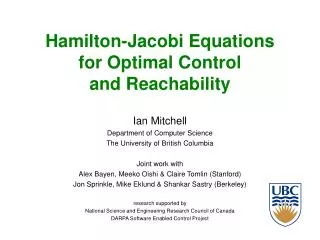
Hamilton-Jacobi Equations for Optimal Control and Reachability. Ian Mitchell Department of Computer Science The University of British Columbia Joint work with Alex Bayen, Meeko Oishi & Claire Tomlin (Stanford) Jon Sprinkle, Mike Eklund & Shankar Sastry (Berkeley) research supported by

E N D
Hamilton-Jacobi Equationsfor Optimal Controland Reachability Ian Mitchell Department of Computer Science The University of British Columbia Joint work with Alex Bayen, Meeko Oishi & Claire Tomlin (Stanford) Jon Sprinkle, Mike Eklund & Shankar Sastry (Berkeley) research supported by National Science and Engineering Research Council of Canada DARPA Software Enabled Control Project
Outline • Dynamic programming for discrete time optimal control • Hamilton-Jacobi equation for continuous time optimal control • Formal derivation • Time-dependent vs static • Viscosity solution concepts • Hamilton-Jacobi equation for reachability • Characterization of backwards reach tube • Examples and applications • Dimensional reduction through projection Ian Mitchell (UBC Computer Science)
Dynamic Programming in Discrete Time • Consider finite horizon objective with = 1 (no discount) • So given u(¢) we can solve inductively backwards in time for objective J(t, x, u(¢)), starting at t = tf • Called dynamic programming (DP) Ian Mitchell (UBC Computer Science)
Optimal Control via Dynamic Programming • DP can also be applied to the value function • Second step works because u(t0) can be chosen independently of u(t) for t > t0 Ian Mitchell (UBC Computer Science)
Optimal Control via Dynamic Programming • Optimal control signal u*(¢) • Observe update equation • Can be extended (with appropriate care) to • other objectives • probabilistic models • adversarial models Ian Mitchell (UBC Computer Science)
Discrete Time LQR • Stephen Boyd’s class at Stanford: EE363 Linear Dynamical Systems: http://www.stanford.edu/class/ee363/ • Discrete LQR: lecture notes 1 • pages 1-1 to 1-4 (from 2005): LQR background • pages 1-13 to 1-16 (from 2005): Dynamic programming sol’n • pages 1-19 to 1-23 (from 2005): HJ equation for LQR Ian Mitchell (UBC Computer Science)
Continuous Time LQR • Stephen Boyd’s class at Stanford: EE363 Linear Dynamical Systems: http://www.stanford.edu/class/ee363/ • Continuous LQR: lecture notes 4 • pages 4-1 to 4-9 (from 2005): derivation of HJ (and Riccati differential equation) via discretization Ian Mitchell (UBC Computer Science)
Outline • Dynamic programming for discrete time optimal control • Hamilton-Jacobi equation for continuous time optimal control • Formal derivation • Time-dependent vs static • Viscosity solution concepts • Hamilton-Jacobi equation for reachability • Characterization of backwards reach tube • Examples and applications • Dimensional reduction through projection Ian Mitchell (UBC Computer Science)
Dynamic Programming Principle • Target set problem • Value function (x) is “cost to go” from x to the nearest target • Value (x) at a point x is the minimum over all points y in the neighborhood N(x) of the sum of • the value (y) at point y • the cost c(x!y) to travel from x to y • Dynamic programming applies if • Costs are additive • Subsets of feasible paths are themselves feasible • Concatenations of feasible paths are feasible Ian Mitchell (UBC Computer Science)
Continuous Dynamic Programming Ian Mitchell (UBC Computer Science)
Static Hamilton-Jacobi PDE Ian Mitchell (UBC Computer Science)
Hamilton-Jacobi Flavours • Stationary (static/time-independent) Hamilton-Jacobi used for target based cost to go and time to reach problems • PDE coupled to boundary conditions • Solution may be discontinuous • Time-dependent Hamilton-Jacobi used for dynamic implicit surfaces and finite horizon optimal control / differential games • PDE coupled to initial/terminal and possibly boundary conditions • Solution continuous but not necessarily differentiable • Other versions exist • Discounted and/or infinite horizon Ian Mitchell (UBC Computer Science)
Time-Dependent Hamilton-Jacobi PDE Ian Mitchell (UBC Computer Science)
Time-Dependent Hamilton-Jacobi PDE Ian Mitchell (UBC Computer Science)
Time-Dependent Hamilton-Jacobi PDE • Finite horizon problem value function defined by • From t = tf, we get PDE with terminal conditions • A very informal derivation of the time-dependent Hamilton-Jacobi equation • Rigourous derivations must account for (t, x) not differentiable, the optimal u(¢) may not exist, … • Resolution: viscosity solutions Ian Mitchell (UBC Computer Science)
Viscosity Solutions • Hamilton-Jacobi PDE for optimal control derived by Bellman in 1950s, but in general there is no classical solution • Even if dynamics f and cost functions g and gf are smooth, solution may not be differentiable • Early attempt to define a weak solution: “vanishing viscosity” • Take limit as ε→ 0 of solution to • Unfortunately, limit may not exist • Crandall & Lions (1983) propose “viscosity solution” • Under reasonable conditions there exists a unique solution • If there exists a classical solution, then it is the same as the viscosity solution • If there exists a vanishing viscosity solution, then it is the same as the viscosity solution • Not the only possible weak solution, but it is the right one for control and reachability Ian Mitchell (UBC Computer Science)
Viscosity Solution Definition • Original definition no longer used • More common definition from Crandall, Evans & Lions (1984) • Solution (t, x) satisfies terminal conditions • For each smooth test function (t, x) • Solution satisfies a comparison principle • If and solve the same HJ PDE where ≥ on the boundary (including initial or terminal times), then ≥ everywhere • Comparison principles are now the preferred way of characterizing viscosity solutions for PDEs Ian Mitchell (UBC Computer Science)
Viscosity Solution Citations • Since extended to • Discounted infinite horizon • Static (for minimum cost to go) • Two player zero sum games • Degenerate elliptic (for SDE dynamics) • Citations: • Evans & Souganidis (1984) for differential games • Crandall, Ishii & Lions (1992) “User’s guide” (dense reading) • Viscosity Solutions & Applications Springer’s Lecture Notes in Mathematics (1995), featuring Bardi, Crandall, Evans, Soner & Souganidis (Capuzzo-Dolcetta & Lions eds) • Optimal Control & Viscosity Solutions of Hamilton-Jacobi-Bellman Equations, Bardi & Capuzzo-Dolcetta (1997) Ian Mitchell (UBC Computer Science)
Outline • Dynamic programming for discrete time optimal control • Hamilton-Jacobi equation for continuous time optimal control • Formal derivation • Time-dependent vs static • Viscosity solution concepts • Hamilton-Jacobi equation for reachability • Characterization of backwards reach tube • Examples and applications • Dimensional reduction through projection Ian Mitchell (UBC Computer Science)
Calculating Reach Sets • Two primary challenges • How to represent set of reachable states • How to evolve set according to dynamics • Discrete systems xk+1 = (xk) • Enumerate trajectories and states • Efficient representations: Binary Decision Diagrams • Continuous systems dx/dt = f(x)? Ian Mitchell (UBC Computer Science)
Implicit Surface Functions • Set G(t) is defined implicitly by an isosurface of a scalar function (x,t),with several benefits • State space dimension does not matter conceptually • Surfaces automatically merge and/or separate • Geometric quantities are easy to calculate • Set must have an interior • Examples (and counter-examples) shown on board Ian Mitchell (UBC Computer Science)
Reachable Set as Optimal Control • Represent the target set as an implicit surface function • Solve an optimal control problem with target set implicit surface function as the terminal cost, and zero running cost • Resulting value function is an implicit surface function for the backward reach set Ian Mitchell (UBC Computer Science)
y vp a q x ve 5 b evader aircraft (control) pursuer aircraft (disturbance) Game of Two Identical Vehicles • Classical collision avoidance example • Collision occurs if vehicles get within five units of one another • Evader chooses turn rate |a| ≤ 1 to avoid collision • Pursuer chooses turn rate |b| ≤ 1 to cause collision • Fixed equal velocity ve=vp = 5 dynamics (pursuer) Ian Mitchell (UBC Computer Science)
y vp a x ve b evader aircraft (control) pursuer aircraft (disturbance) Collision Avoidance Computation • Work in relative coordinates with evader fixed at origin • State variables are now relative planar location (x,y) and relative heading target set description Ian Mitchell (UBC Computer Science)
Evolving Reachable Sets • Modified Hamilton-Jacobi partial differential equation growth of reachable set final reachable set Ian Mitchell (UBC Computer Science)
Solving a Differential Game • Terminal cost differential game for trajectories f(¢; x,t,a(¢),b(¢)) • Value function solution (x,t) given by viscosity solution to basic Hamilton-Jacobi equation • [Evans & Souganidis, 1984] Ian Mitchell (UBC Computer Science)
Modification for Optimal Stopping Time • How to keep trajectories from passing through G(0)? • [Mitchell, Bayen & Tomlin, IEEE T. Automatic Control, 2005] • Augment disturbance input • Augmented Hamilton-Jacobi equation solves for reachable set • Augmented Hamiltonian is equivalent to modified Hamiltonian Ian Mitchell (UBC Computer Science)
Application: Collision Alert for ATC • Use reachable set to detect potential collisions and warn Air Traffic Control (ATC) • Find aircraft pairs in ETMS database whose flight plans intersect • Check whether either aircraft is in the other’s collision region • If so, examine ETMS data to see if aircraft path is deviated • One hour sample in Oakland center’s airspace— • 1590 pairs, 1555 no conflict, 25 detected conflicts, 2 false alerts Ian Mitchell (UBC Computer Science)
Application: Synthesizing Safe Controllers • By construction, on the boundary of the unsafe set there exists a control to keep trajectories safe • Filter potentially unsafe controls to ensure safety by construction continuous system dynamics n(x1) x1 G(0) G(t) G(t) Ian Mitchell (UBC Computer Science)
safety filter’s input modification evader’s actual input collision set reachable set (unsafe set) evader pursuer evader’s desired input pursuer’s input Synthesizing Safe Controls (No Safety) • Use reachable sets to guarantee safety • Basic Rules • Pursuer: turn to head toward evader • Evader: turn to head east • No filtering of evader input Ian Mitchell (UBC Computer Science)
safety filter’s input modification evader’s actual input collision set reachable set (unsafe set) evader pursuer evader’s desired input pursuer’s input Synthesizing Safe Controls (Success) • Use reachable sets to guarantee safety • Basic Rules • Pursuer: turn to head toward evader • Evader: turn to head east • Evader’s input is filtered to guarantee that pursuer does not enter the reachable set Ian Mitchell (UBC Computer Science)
safety filter’s input modification evader’s actual input collision set reachable set (unsafe set) evader pursuer evader’s desired input pursuer’s input Synthesizing Safe Controls (Failure) • Use reachable sets to guarantee safety • Basic Rules • Pursuer: turn to head toward evader • Evader: turn to head east • Evader’s input is filtered, but pursuer is already inside reachable set, so collision cannot be avoided Ian Mitchell (UBC Computer Science)
Acoustic Capture • Modified version of homicidal chauffeur from [Cardaliaguet, Quincampoix & Saint-Pierre, 1999] • Pursuer is faster with limited turn radius but fast rotation • Evader can move any direction, but speed is lowered near pursuer • Also solved in relative coordinates continuous system dynamics Ian Mitchell (UBC Computer Science)
Application: Glideslope Recapture • safe-set of operation relative to the desired point of landing on the virtual runway (f) • vector-off maneuver requested • command to land (if possible) is given • aircraft will continue to vector-off (if landing is unsafe) or will issue commands to recapture the glideslope at some point (e) Ian Mitchell (UBC Computer Science)
Simple Model, Use Some Tricks • Aircraft acts like a kinematic cart in longitudinal and lateral dynamics • Reduce 5D state space to two 2D calculations • Separate (x,y,) and (x,z,) calculations • Swap integration variable t to x • Variable resolution grid (two methods) • [Sprinkle, Eklund & Sastry, Proc. ACC, 2005] • [Sprinkle, Ames, Eklund, Mitchell & Sastry, Innovations in Systems & Software Engineering, 2005] Ian Mitchell (UBC Computer Science)
Implementation and Results • ACC results shown; ISSE results difficult to visualize • All pieces fit together, grid resolution changes by factor of ten • ISSE uses nonlinear coordinate transform to avoid the need for separate grids [0,3) [3,10) Ian Mitchell (UBC Computer Science)
Implementation and Results [1,3) [3,10) [0,1) Ian Mitchell (UBC Computer Science)
Implementation • Use backward reach set to make one lookup table for each projection • ~7MB total size • Lookup time: ~10ms (~5ms each) • Time to generate: • ~15 mins for the reach set • ~2 hours to compile into an executable (due to compiler issues) • Additional issues • Smooth control laws • Decision delay • Total development time • ~2 man months of coding, plus design and research required for safe sets Ian Mitchell (UBC Computer Science)
Demonstration & Results • Flown on live T-33 aircraft • Landing on “virtual” runway at a high altitude • Ground controller gives vector-off and recapture commands • 1 successful landing • 1 go-around after “unsafe” answer (later verified offline as a correct result) Ian Mitchell (UBC Computer Science)
Projective Overapproximation • Overapproximate reachable set of high dimensional system as the intersection of reachable sets for lower dimensional projections • [Mitchell & Tomlin, 2002] • Example: rotation of “sphere” about z-axis Ian Mitchell (UBC Computer Science)
Computing with Projections • Forward and backward reachable sets for finite automata • Projecting into overlapping subsets of the variables, computing with BDDs [Govindaraju, Dill, Hu, Horowitz] • Forward reachable sets for continuous systems • Projecting into 2D subspaces, representation by polygons [Greenstreet & Mitchell] • Level set algorithms for geometric optics • Need multiple arrival time (viscosity solution gives first arrival time), so compute in higher dimensions and project down [Osher, Cheng, Kang, Shim & Tsai] Ian Mitchell (UBC Computer Science)
Hamilton-Jacobi in the Projection • Consider x-z projection represented by level set xz(x,z,t) • Back projection into 3D yields a cylinder xz(x,y,z,t) • Simple HJ PDE for this cylinder • But for cylinder parallel to y-axis, p2 = 0 • What value to give free variable y in fi(x,y,z)? • Treat it as a disturbance, bounded by the other projections • Hamiltonian no longer depends on y, so computation can be done entirely in x-z space on xz(x,z,t) Ian Mitchell (UBC Computer Science)
Projective Collision Avoidance • Work strictly in relative x-y plane • Treat relative heading [ 0, 2p ] as a disturbance input • Compute time: 40 seconds in 2D vs 20 minutes in 3D • Compare overapproximative prism (mesh) to true set (solid) Ian Mitchell (UBC Computer Science)
Projection Choices • Poorly chosen projections may lead to large overapproximations • Projections need not be along coordinate axes • Number of projections is not constrained by number of dimensions good projections poor projections Ian Mitchell (UBC Computer Science)