Download
1 / 23
320 likes | 736 Views
Optimal Control. Motivation Bellman’s Principle of Optimality Discrete-Time Systems Continuous-Time Systems Steady-State Infinite Horizon Optimal Control Illustrative Examples. Motivation. Control design based on pole-placement often has non unique solutions

E N D
Optimal Control • Motivation • Bellman’s Principle of Optimality • Discrete-Time Systems • Continuous-Time Systems • Steady-State Infinite Horizon Optimal Control • Illustrative Examples
Motivation • Control design based on pole-placement often has non unique solutions • Best locations for eigenvalues are difficult to determine • Optimal control minimizes a performance index based on time response • Control gains result from solving the optimal control problem
Quadratic Functions Single variable quadratic function: Multi-variable quadratic function: Where Q is a symmetric (QT=Q) nxn matrix and b is an nx1 vector It can be shown that the Jacobian of f is
2-Variable Quadratic Example Quadratic function of 2 variables: Matrix representation:
Quadratic Optimization The value of x that minimizes f(x) (denoted by x*) sets or equivalently Provided that the Hessian of f, is positive definite
Positive Definite Matrixes Definition: A symmetric matrix H is said to be positive definite (denoted by H>0) if xTHx>0 for any non zero vector x (semi positive definite if it only satisfies xTHx0 for any x (denoted by H 0) ). Positive definiteness (Sylvester) test: H is positive definite iff all the principal minors of H are positive:
2-Variable Quadratic Optimization Example Optimal solution: Thus x* minimizes f(x)
Discrete-Time Linear Quadratic (LQ) Optimal Control Given discrete-time state equation Find control sequence u(k) to minimize
Comments on Discrete-Time LQ Performance Index (PI) • Control objective is to make x small by penalizing large inputs and states • PI makes a compromise between performance and control action uTRu xTQx t
Principle of Optimality 4 2 7 5 9 1 3 8 6 Bellman’s Principle of Optimality: At any intermediate state xi in an optimal path from x0 to xf, the policy from xi to goal xf must itself constitute optimal policy
Discrete-Time LQ Formulation Optimization of the last input (k=N-1): Where x(N)=Gx(n-1)+Hu(n-1). The optimal input at the last step is obtained by setting Solving for u(N-1) gives
Optimal Value of JN-1 Substituting the optimal value of u(N-1) in JN gives The optimal value of u(N-2) may be obtained by minimizing where But JN-1 is of the same form as JN with the indexes decremented by one.
Summary of Discrete-Time LQ Solution Control law: Ricatti Equation Optimal Cost:
Comments on Continuous-Time LQ Solution • Control law is a time varying state feedback law • Matrix Pk can be computed recursively from the Ricatti equation by decrementing the index k from N to 0. • In most cases P and K have steady-state solutions as N approaches infinity
Matlab Example y Find the discrete-time (T=0.1) optimal controller that minimizes u M=1 Solution: State Equation
Discretized Equation and PI Weighting Matrices Discretized Equation: Performance Index Weigthing Matrices: R Q PN
System Definition in Matlab %System: dx1/dt=x2, dx2/dt=u %System Matrices Ac=[0 1;0 0]; Bc=[0;1]; [G,H]=c2d(Ac,Bc,0.1); %Performance Index Matrices N=100; PN=[10 0;0 0]; Q=[1 0;0 0]; R=2;
Ricatti Equation Computation %Initialize gain K and S matrices P=zeros(2,2,N+1); K=zeros(N,2); P(:,:,N+1)=PN; %Computation of gain K and S matrices for k=N:-1:1 Pkp1=P(:,:,k+1); Kk=(R+H'*Pkp1*H)\(H'*Pkp1*G); Gcl=G-H*Kk; Pk=Gcl'*Pkp1*Gcl+Q+Kk'*R*Kk; K(k,:)=Kk; P(:,:,k)=Pk; end
LQ Controller Simulation %Simulation x=zeros(N+1,2); x0=[1;0]; x(1,:)=x0'; for k=1:N xk=x(k,:)'; uk=-K(k,:)*xk; xkp1=G*xk+H*uk; x(k+1,:)=xkp1'; end %plot results
Linear Quadratic Regulator Given discrete-time state equation Find control sequence u(k) to minimize Solution is obtained as the limiting case of Ricatti Eq.
Summary of LQR Solution Control law: Ricatti Equation Optimal Cost: