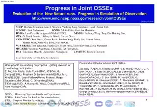
Simulation of observation and calibration for Joint OSSEs

1. Simulation of observation and calibration for Joint OSSEs Jack S. Woollen[1,+], Michiko Masutani[1,2,#], Tong Zhu[4,@], Nikki Prive[4,@], Yuanfu Xie[4], Lars Peter Riishojgaard, [2,$,5], David Groff[1,+], Ronald L. Vogel[1,+], Thomas J. Kleespies[3], Harper Pryor [5,+] , Ellen Salmon[5,+] [1]NOAA/National Centers for Environmental Prediction (NCEP) [2]Joint Center for Satellite and Data Assimilation (JCSDA) [3]NOAA/ NESDIS/STAR, [4]NOAA/Earth System Research Laboratory (ESRL) [5] NASA/GSFC # Wyle Information Systems, McLean, VA, +Science Applications International Corporation (SAIC), MD $Goddard Earth Science and Technology Center, University of Maryland, Baltimore, MD, @Cooperative Institute for Research in the Atmosphere (CIRA)/CSU, CO

2. Full OSSEs There are many types of simulation experiments. Sometimes, we have to call our OSSE a ‘Full OSSE’ to avoid confusion. Advantages • A Nature Run (NR, proxy true atmosphere) is produced from a free forecast run using the highest resolution operational model which is significantly different from NWP model used in DAS. • Calibrations will be performed to provide quantitative data impact assessment. • Data impact on analysis and forecast will be evaluated. • A Full OSSE can provide detailed quantitative evaluations of the configuration of observing systems. • A Full OSSE can use an existing operational system and help the development of an operational system . compare data impacts between real and simulated data will be performed. Without calibration quantitative evaluation of data impact is not possible. OSSE Calibration ● In order to conduct calibration all major existing observation have to be simulated. ●The calibration includes adjusting observational error. ●If the difference is explained, we will be able to interpret the OSSE results as to real data impact. ●The results from calibration experiments provide guidelines for interpreting OSSE results on data impact in the real world. ●Without calibration, quantitative evaluation data impact using OSSE could mislead the meteorological community. In this OSSE, calibration was performed and presented. Existing Data assimilation system and vilification method are used for Full OSSEs. This will help development of DAS and verification tools. International Joint OSSE capability • Full OSSEs are expensive • Sharing one Nature Run and simulated observation save the cost • Share diverse resources • OSSE-based decisions have international stakeholders • Decisions on major space systems have important scientific, technical, financial and political ramifications • Community ownership and oversight of OSSE capability is important for maintaining credibility • Independent but related data assimilation systems allow us to test robustness of answers

3. New Nature Run by ECMWF Based on discussion with JCSDA, NCEP, GMAO, GLA, SIVO, SWA, NESDIS, ESRL, and ECMWF Two High Resolution Nature Runs 35 days long Hurricane season: Starting at 12z September 27,2005, Convective precipitation over US: starting at 12Z April 10, 2006 T799 resolution, 91 levels, one hourly dump Get initial conditions from T511 NR Not recommended for OSSE Joint OSSE Nature Run Spectral resolution : T511 Vertical levels: L91 3 hourly dump Initial conditions: 12Z May 1st, 2005 Ends at: 0Z Jun 1,2006 Daily SST and ICE: provided by NCEP Model: Version cy31r1 T511 Nature Run is found to be representative of the real atmosphere and suitable for conducting reliable OSSEs for midlatitude systems and tropical cyclones. (Note: MJO in T511 Nature Run is still weak.) There are significant developments in high resolution forecast models at ECMWF since 2006 and a more realistic tropics for T799 Nature Run is expected with a newer version of the ECMWF model. ECMWF agreed to generate a new T799 NR, when the Joint OSSE team has gained enough experience in OSSEs with T511NR and is ready to make the best use of the high resolution Nature Run. For the time being, the Joint OSSE team will concentrate on OSSEs using the T511 Nature Run. Note: This data must not be used for commercial purposes and re-distribution rights are not given. User lists are maintained by Michiko Masutani and ECMWF Supplemental low resolution regular lat lon data 1degx1deg for T511 NR Pressure level data:31 levels, Potential temperature level data: 315,330,350,370,530K Selected surface data for T511 NR:

4. Data Sharing in Joint OSSEs Archive and Distribution of the Nature Run Simulated observation and other useful data will be shared among Joint OSSE teams. NASA/NCCS provided dis space for Joint OSSE data sharering There is a entry created for Joint OSSE http://portal.nccs.nasa.gov/josse/index.pl Make entry to each data set and generating institute, and contact person. People use these data must contact generating institutes. To be archived in the MARS system at ECMWF Accessed by external users. Currently available internally as expver=etwu • Copies for US are available to designated users for research purpose& users known to ECMWF • Saved at NCEP, ESRL, and NASA/GSFC • Complete data available from portal at NASA/GSFC • Conctact:Michiko Masutani (michiko.masutani@noaa.gov), Harper.Pryor@nasa.gov • Gradsdods access is available for T511 NR. The data can be down loaded  in grib1, NetCDF, binary. The data can be retrieved globally or selected region. • Provide IP number to :Arlindo da Silva (Arlindo.Dasilva@nasa.gov)

5. Flexile Radiance data Simulation strategies at NCEP-NESDIS Progress and current plan Simulation of observational data for calibration ► Ozone data from SBUV ► Conventional data based on NCEP reanalysis quality controlled distribution. (More complete data set compared to operational data) ► Satellite radiance data in 2005 distribution. AMSUA, AMSUB, GOES, HIRS2, HIRS3, AIRS,MSU are being generated at foot print used by NCEP operational analysis. ► Observational error is random error based on error table. ► Limited calibration and validation will be conducted by NCEP and NESDIS for their own use. However, users are expected to perform their own calibrations and validation. The DBL91 also used for development of RTM. DBL91 can be processed for other sampling such as GMAO sampling DBL91 can be processed for new observation DWL91 with sampling based on GDAS usage will be posted from NASA portal. It is an option whether DBL91 to be saved and exchange among various project, or DBL91 to be treated as temporary file produced in simulation process. This depends on size of DBL91 compare to the Nature Run. Future Plan ► Observational error based on correlated noise ► Simulation and assimilation of cloudy radiance and let sampling done by assimilation. Cloudy radiance is still under development

6. DBL91 • Nature Run data at foot print • 91 level 3-D data (12 Variables) • 2-D data (71 Variables) • Climatological data • All information to simulate Radiances NR 91 levels of: pres cloudcov cloudice cloudh2o ozone mmr temperature spfhumid From BUFR satellite file 2005.00 004001 YEAR YEAR YEAR 5.00 004002 MNTH MONTH MONTH 1.00 004003 DAYS DAY DAY 21.00 004004 HOUR HOUR HOUR .00 004005 MINU MINUTE MINUTE 3.00 004006 SECO SECOND SECOND 168.67 006002 CLON DEGREES LONGITUDE 59.77 005002 CLAT DEGREES LATITUDE 206.00 001007 SAID CODE TABLE SAT IDENTIFIER 570.00 002019 SIID CODE TABLE SAT INSTRUMENTS 2.00 005043 FOVN NUMERIC BEAM POSITION 1.00 008012 LSQL CODE TABLE LAND/SEA QUALIFIER 52.79 007024 SAZA DEGREE SAT ZENITH ANGLE 59.83 007025 SOZA DEGREE SOLAR ZENITH ANGLE .00 010001 HOLS METER HEIGHT OF LAND SURFACE 813000.00 007002 HMSL METER HEIGHT OR ALTITUDE From NCEP Climatology .00000 iv=27 ! low vegetation cover .00000 iv=28 ! high vegetation cover .00000 iv=29 ! low vegetation type .00000 iv=30 ! high vegetation type Surface quantities from Nature Run 31 1 Sea-ice cover [(0-1)] 32 2 Snow albedo [(0-1)] 33 3 Snow density [kg m**-3] 34 4 Sea surface temperature [K] 44 5 Snow evaporation [m of water] 45 6 Snowmelt [m of water] 50 7 Large-scale precipitation fraction [s] 57 8 Downward uv radiation at the surface [w m**-2 s] 58 9 Photosynthetically active radiation [w m**-2 s] 59 10 Convective available potential energy [J kg**-1] 78 11 Total column liquid water [kg m**-2] 79 12 Total column ice water [kg m**-2] 129 13 Geopotential [m**2 s**-2] 136 14 Total column water [kg m**-2] 137 15 Total column water vapour [kg m**-2] 141 16 Snow depth [m of water equivalent] 142 17 Stratiform precipitation [m] 143 18 Convective precipitation [m] 144 19 Snowfall (convective + stratiform) [m of water equ 145 20 Boundary layer dissipation [W m**-2 s] 146 21 Surface sensible heat flux [W m**-2 s] 147 22 Surface latent heat flux [W m**-2 s] 148 23 Charnock 151 24 Mean sea-level pressure [Pa] 152 25 Surface pressure {pa] 159 26 Boundary layer height [m] 164 27 Total cloud cover [(0 - 1)] 165 28 10 metre U wind component [m s**-1] 166 29 10 metre V wind component [m s**-1] 167 30 2 metre temperature [K] 168 31 2 metre dewpoint temperature [K] 169 32 Surface solar radiation downwards [W m**-2 s] 172 33 Land/sea mask [(0, 1)] 175 34 Surface thermal radiation downwards [W m**-2 s] 176 35 Surface solar radiation [W m**-2 s] 177 36 Surface thermal radiation [W m**-2 s] 178 37 Top solar radiation [W m**-2 s] 179 38 Top thermal radiation [W m**-2 s] 180 39 East/West surface stress [N m**-2 s] 181 40 North/South surface stress [N m**-2 s] 182 41 Evaporation [m of water] 186 42 Low cloud cover [(0 - 1)] 187 43 Medium cloud cover [(0 - 1)] 188 44 High cloud cover [(0 - 1)] 189 45 Sunshine duration [s] 195 46 Lat. component of gravity wave stress [N m**-2 s] 196 47 Meridional component of gravity wave stress [N m** 197 48 Gravity wave dissipation [W m**-2 s] 198 49 Skin reservoir content [m of water] 205 50 Runoff [m] 206 51 Total column ozone [Dobson] 208 52 Top net solar radiation, clear sky [W m**-2] 209 53 Top net thermal radiation, clear sky [W m**-2] 210 54 Surface net solar radiation, clear sky [W m**-2] 211 55 Surface net thermal radiation, clear sky [W m**-2] 235 56 Skin temperature [K] 238 57 Temperature of snow layer [K] 243 58 Forecast albedo [(0 - 1)] 244 59 Forecast surface roughness [m] 245 60 Forecast log of surface roughness for heat Experts for data handling and experts of RTM are different people. The DBL91 also used for development of RTM. DBL91 can be processed for other sampling such as GMAO sampling DBL91 can be processed for new observation It is an option whether DBL91 to be saved and exchange among various project, or DBL91 to be treated as temporary file produced in simulation process. This depends on size of DBL91 compare to the Nature Run.

7. Simulation of AMSU-A/BTong Zhu (NESDIS) Simulation of HIRS3 radiance from NOAA16 M Masutani (NCEP) • AMSU-A on NOAA15 and 16, AMSU-B on NOAA15, 16, and 17 radiances were simulated for the same 13 months. • 6-Hourly radiance data has been simulated, with the data coverage consistent with the operational GSI data ingest time. • Update the simulation by using NR output ice coverage data. • Angular dependences and channel correlations have been calculated. More validation study is necessary. Latest version of CRTM (1.2.2) is used for simulation DBL 91 was generated at foot print used by NCEP GDAS All information in GDAS bufr files are copied to simulated radiance file. Channel which are not used by GDAS was marked in diag file. Masked out to generate masked radiance data. Comparison With Observation 1800 UTC 31 May 2005 Template data Observed radiance with horizontal thinning Horizontal and vertical thinning Simulation Observation Horizontal thinning HIRS3 NOAA 16 Ch=4 May 2nd 00z (f12)

8. Simulation GOES Radiance for OSSETong Zhu (CIRA/CSU), Fuzhong Weng (NOAA/NESDIS), Michiko Masutani (NOAA/EMC), Steve Load (NOAA/EMC), Jack Woollen (NOAA/EMC), Thomas J. Kleespies(NOAA/NESDIS), Yong Han(NOAA/NESDIS), Quanhua, Liu (QSS), Sid Boukabara (NOAA/NESDIS) Advanced Baseline Imager (ABI) will be flown on the next generation of NOAA Geostationary Operational Environmental Satellite (GOES)-R platform. The sensor will provide enhanced spatial, temporal information for atmospheric moisture, wind and many surface properties. A joint Observation System Simulation Experiments (OSSE) project was started recently to study the impacts of GOES-R ABI measurements on numerical weather prediction. In this poster, we will present some results of the simulation of GOES radiances based on OSSE nature run output and the evaluation against observations. A case study will be performed to analysis ECMWF T511 natural run results. ABI instrument properties and geometry factors are simulated based on current GOES and MSG SEVIRI sensors. The JCSDA Community Radiative Transfer Model (CRTM) is used to simulate ABI radiances with the natural run atmospheric profiles. The simulated radiances are evaluated by comparing with current GOES observations. Current GOES Imager IR band has 4 km horizontal resolution (FOV), GOES Sounder has 10 km resolution. A full disk scan has total 10,080,910 observation points, and takes about 26 min. GOES-R ABI sensor will has 1km/2 km resolution. Steps: 1. The OSSE Nature Run data is come from ECMWF T511 13-month simulation. The data set contains 91 vertical levels variables, which are then horizontally interpolated to observation points without vertical interpolation. Selected model level data and all surface data are included. 2. CRTM model is used to simulate GOES-12 Imager, Sounder, MSG SEVIRI, and GOES-R ABI measurements. 3. Perform validations of the simulated radiances with statistical analysis and comparison with real observations. Radiance Simulation Design Objective GOES data is simulated to test impact of GOES in simulation experiments in comparison with impact of real data. OSSE for GOES will serve as a calibration for GOESR OSSE. GOES-EAST Observation Locations Radiance Simulation Flow Chart A full disk scan of GOES-12 Imager has total 10,080,910 observation points with 4 km resolution. However, Current NCEP/GSI model only take a thinned 1x1 degree GOES-12 dataset. In this study, we extract GOES-12 Imager observation locations (lon/lat) at 20 km and 60 km resolutions. The Nature Run data is interpolated on to these two different resolution locations. Reduced to ~20 km, 403239 points Reduced to ~60 km, 40323 points

9. Time Series of Mean Tb Simulation of GOES-12 Sounder Simulation of GOES-12 Imager Simulated GOES-12 Imager 4 bands with ECMWF Nature Run output data at 0300 UTC October 1, 2005. It is found that the water vapor band, 6.5 µm, is most accurate band simulated by CRTM model. Simulated Radiances Observed vs. simulated GOES-12 sounder for the mean Tb over North Atlantic Ocean region.Black lines are mean Tb from NR simulated, and the red lines are the mean Tb from observation. They should not be the same but similar statistical features are important. In nature Run, there is hurricane generated on September 27. At 1200 UTC October 1, it is located at about 43 W, 20N. The high moisture air mass associated with the hurricane is shown clearly. Progress Time series of hourly, full disk mean brightness temperature of the simulated GOES-12 Imager 4 bands from September 28 to October 10, 2005.Under clear sky conditions, the brightness temperatures are warmer than that of cloudy conditions. The daily change under clear conditions is apparent. The observed GOES-12 Sounder Preliminary simulation of GOES from T511NR has completed for entire Nature Run period (13 month) Observed GOES-12 18 bands on 0230 UTC October 01, 2005 for North Atlantic Ocean section. Future Work Simulate GOES-R ABI radiances from Nature Run data,Perform NWP model simulations to investigate the impacts of GOES-12 and GOES-R measurements. Conduct impact test using data assimilation system Black lines are total points mean Tb, red lines are the mean Tb over clear sky condition, and the blue lines are the mean Tb over cloudy condition. Clear sky condition is defined as where total cloud coverage (TCC)< 0.1, and cloudy condition is where TCC > 0.1 Time Series of Mean Tb Time Series of Mean Tb Time Series of Mean Tb Time Series of Mean Tb

10. Simulated SBUV Ozone Retrievals Jack Woollen(NCEP) • OSSE Observation Simulation and Experiment Verification • Developments • Jack Woollen (NCEP) • New simulation of run history PREPQC files with QC information • Simulation of SBUV BUFR ozone observations • Create simulated BUFR AMSUa, AMSUb, and GOES files (w/Tong Zhu) • Updated version of DBL91 files produced with GSI h/v thinning info • Optimized experiment cycle script provides 15:1 production speedup • Suru fit files/plots adapted for OSSE calibration experiments • Scatter fit plots developed for experiment comparisons • Radiance fit plots to examine results of bias correction experiments Simulating the SBUV retrievals involves converting the 91 level ozone concentrations from the nature run into 12 layers of ozone amounts (DU). The plot checks the conversion by comparing the NR total ozone values with the total profile ozone derived by summing the simulated layer values.

11. OSSE Calibration Progress in Calibration at ESRL-NCEP • ESRL and NCEP are working on calibration using data denial method and fits to observation. • Using simulated data by GMAO and additional data from NCEP. • Focused on July-August 2005. • GSI version May 2007. • NCEP is working on upgrading OSSE system to newer GSI to accommodate DWL and flow dependent error covariances. Some calibrations will be repeated. ● In order to conduct calibration all major existing observation have to be simulated. ●The calibration includes adjusting observational error. ●If the difference is explained, we will be able to interpret the OSSE results as to real data impact. ●The results from calibration experiments provide guidelines for interpreting OSSE results on data impact in the real world. ●Without calibration, quantitative evaluation data impact using OSSE could mislead the meteorological community. In this OSSE, calibration was performed and presented. • Data denial tests are run for synthetic obs subsets of similar data types • Analysis impact (global RMS difference in control and data denial analysis) is calculated for synthetic obs and compared to analysis impact for data denial with real archived data from July 2005 • Standard deviation of synthetic errors are adjusted, errors are regenerated • New data denial case is run and compared to real data, errors adjusted, etc • Repeat until analysis impact matches real data analysis impact, or until satisfied that calibration is not possible

12. A Calibration Example (RAOB) Nikki Prive, YuanfuXsi (ESRL) • All RAOB/sonde types (120, 132, 182, 220 232) simultaneously tested. Error standard deviation adjusted at individual height levels for each obs type (T, RH, wind). • RH and Wind most successfully calibrated. • T is reasonably but not ‘perfectly’ calibrated. • Some levels were not able to be calibrated: T below 800 mb, above 150 mb Q above 250 mb Wind above 100 mb Successful calibration Calibration not needed Calibration not possible

13. Fit files storage and display Jack Woollen (NCEP) NCEP operational fit files contain rms, means, and counts of ob-bg Seven regions: GL, NH, SH, TR, NA, EU, AS RAOB ps, 21 levels of q,t,u,v,z, 7 regions SURF ps from adpsfc and sfcshp, 7 regions ACFT t,z,u,v,spd, 1000-700,700-300,300-150, 7 regions ACAR t,z,u,v,spd, 1000-700,700-300,300-150, NA only Filenames have the form fnn.type.date, ie f00.raob.2005070100 Each file has fits for 1 lead time, 1 datatype, 7 regions, 1 valid time GRADS combines these files to produce time series or scatter fit plots Suru plots create f00,f06,f12,f24,f36,f48 for raob surf acft acar .5 MB contains the complete set of Suru fit files for 1 year

14. Scatter Fit Comparison Plots Jack Woollen (NCEP) Need to compare two experiments – use scatter plot Compare all levels and forecast lengths for each variable Comparison with real data case is relevant for calibration Forecast lengths out to 5 days or more can be added Develop a simple way to denote levels and forecast length Analysis and Forecast fit scatter plot comparison with realn Fits between each calibration run are compared with the realn case on a scatter plot. Each dot compares two global average RMS fits for 1 variable, 1 forecast length, one level, and one synoptic time. Dots are plotted for every case where the realn run coincides in space/time with a calibration run. Summary of Calibration Experiments realn - real data run, 3jul-15jul perfn - perfect data run, 22jun-15jul cnverr - simulated data with small errors, 1jul-18jul raob5 - simulated data with bigger raob errors, 1jul-18jul stnob - like cnverr w/sat bias correction initially zero, 22jun-22jul gsitest - like raob5 with modified GSI error specs, 1jul-18jul synth - simulated perfect data but w/o radiosondes, 3jul-15jul synt2 - simulated perfect data, 3jul-15jul Forecast length indicated by dot size - longer length - bigger dot

15. Remark on Joint OSSEs Summary Using Full OSSE, various experiments can be performed and various verification metrics can be tested to evaluate data impact from future instruments and data distributions. It was noted that that while OSSEs can be overly optimistic about the impacts of new observations evaluated in the current data assimilation system, advances in data assimilation skill usually allow us to make better use of observations over time. These advances may, to some extent, be an offsetting factor in that they can help achieve greater impact from new observations in the long run. (From ECMWF Workshop summary) Theoretical predictions have to be confirmed by full OSSEs. The results are often unexpected. OSSE results also require theoretical back ups. OSSE capability should be broadly based (multi-agency) to enhance credibility and to save costs The Nature runs have been posted and made available to research community Initial calibration was conducted using GMAO radiance data and other simulated data at NCEP-NESDIS during July 2005. The initial simulated data will be ready for selected instruments in near future. (target is February 2010) Software to simulation of further radiance system at NCEP-NESDIS are nearly ready. Simulated conventional data and DBL91 has been posted from NASA portal. Comments on OSSE Calibration ●OSSEfunding should include simulation of calibration data and calibration of OSSE. OSSEfunding tends to expect that calibrated OSSEsystem already exists. ● Calibration and simulation of basic observation effort has to be done sharing OSSE resources. ●Without calibration, quantitative evaluation data impact using OSSE could mislead the meteorological community. Acknowledgement The nature runs for Joint OSSEs were produced by Dr. Erik Andersson of ECMWF. We appreciate GMAO to provide initial satellite data for calibration. GMAO also provided code to add random error to simulated data.