Download
1 / 10
100 likes | 104 Views
Cartesian vs. Polar in a Predator-Prey System By Neelesh Shrivastava. Abstract.

E N D
Cartesian vs. Polar in a Predator-Prey System By Neelesh Shrivastava
Abstract This project aims to use an agent-based system to model two different predator-prey systems. The first is in Cartesian x,y, the second is in Polar r,θ. From there, any differences between the predictions of the models will be ascertained.
Background Understanding of different ways to model population and a cursory understanding of the Lotka-Volterra equations is essential to understand population modeling in general. The Lotka-Volterra equations are a set of differential equations governing how population behaves when the two interact with each other. It assumes simple exponential growth/decay for each group, the predator and the prey, and adds a factor to decrease, for the prey, or increase, for the predator, the populations based on interactions between the two populations. Polar and Cartesian are the two most common ways to express coordinates in two dimensions. Cartesian expresses coordinates in terms of x, horizontal distance traveled, and y, vertical distance traveled. Polar expresses coordinates in terms of r, distance from the origin, and θ, counterclockwise angle from the Polar axis, the x-axis in Cartesian.
Procedure Python was be used to implement the simulations and TKinter for a graphical model. Differences, if any, between the Cartesian and Polar models will be found. Because of the way computers handle coordinates, x increases as you move right, but y increases as you move down the screen. Similarly, r increases as you move away from the top left-corner, the origin in cartesian, and theta will increase in a clock-wise direction.
Cartesian Program • Seems to be completely random • Generally, populations get a stable proportion, but because there is no limit on the population of the prey, it just keeps growing
Polar Program • Clear tendency towards the “center”; upper-left and away from the bottom right • Still gets a stable proportion like the Cartesian program • Lack of limit on the prey allows the populations to grow, but it grows at a slower rate than the Cartesian program, on average
Results • Cartesian systems seem random (expected result) • Polar systems result in banded regions that center mostly near the “origin” (in this case, the top-left corner) • Cartesian and Polar systems still keep the same proportions for predators:prey • However, Polar systems generally have lower numbers of total predators and prey.
Conclusion • If the program does not need a graphical component/the positions of the predators and prey are unimportant, the Polar system works fine. • In any case where the position does matter and the system needs to be random, the Cartesian program is needed. • Did not test for directed movement, but based on the results here, Cartesian would work better.
Directed movement, other modifications to the 3D coordinate systems (Cartesian, Cylindrical, Spherical) Other applications which require the use of coordinate systems (anything that requires graphics, projectile motion) Extensions