Download
1 / 121
1.25k likes | 1.32k Views
Example System: Predator Prey Model. https://www.math.duke.edu/education/webfeatsII/Word2HTML/Predator-prey.doc. Example System: Predator Prey Model. Without prey the predators become extinct. Without predators the prey grows unbounded. Populations Oscillate. Chapter 3.

E N D
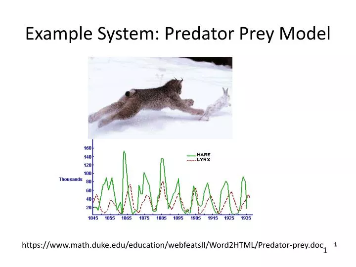
Example System: Predator Prey Model https://www.math.duke.edu/education/webfeatsII/Word2HTML/Predator-prey.doc
Example System: Predator Prey Model Without prey the predators become extinct Without predators the prey grows unbounded Populations Oscillate
Chapter 3 Lyapunov Stability – Autonomous Systems System of differential equations • Question: Is this system “well behaved”? • Follow Up Question: What does well behaved mean? • Do the states go to fixed values? • Do the states stay bounded ? • Do we know limits on the size of the states? • If we could “solve” the system then theses questions may be easy to answer. • We are assuming we can’t solve our systems of interest. Bottom line in this chapter is that we want to know if a differential equation, which we can’t solve, is “well behaved”?
Preview x2 x2 System stops moving, “stable” x1 x1 x(0) x(0) System state grows, “unstable” How can we know which way our system behaves?
No explicit time dependence. The solution will evolve with time, i.e. x(t) Open or closed-loop system • Three main issues: • System is nonlinear • f is a vector • Can’t find a solution Can have multiple equilibrium points We will work to quantify “well behaved”
Starting time (typically 0) Evolution of the state x2 • Khalil calls this the “Challenge and answer form to demonstrate stability” • Challenger proposes an ε bound for the final state • The answerer has to produce a bound on the initial condition so that the state always stays in the εbound. • Answerer has to provide an answer for every ε proposed x1 Bottom line: If we start close enough to xe we stay close to xe
Pendulum without friction. Is (0,0) a stable equilibrium point in the sense of Definition 2? Yes
x(t) goes to xe as t goes to A equilibrium point could be Stable and not Convergent An equilibrium point could be Convergent and Not Stable
Pendulum without friction. Is (0,0) convergent? Is (0,0) asymptotically stable? No No
Pendulum with friction. Is (0,0) a stable equilibrium point in the sense of Definition 2? Is (0,0) convergent? Is (0,0) asymptotically stable? Yes Yes Yes
Includes a sense of “how fast” the system converges. Exponential is “stricter” than asymptotic
Can perform this shift to any equilibrium point of interest (a system may have multiple equilibrium points)
V is a scalar function Notation: PSD write as V0 PD write as V>0 NSD write as V0 ND write as V<0 Could be V(x1(t)) Example: Are each of these PSD, PD, ND, or NSD? V(x1) V(x1) V(x1) V(x1) None ND x1 x1 x1 x1 PD PSD Could be x1(t)
V(x1) Example: x1
Don’t loose generality by restricting Q to be symmetric in quadratic form i.e., Q symmetric See chapter 2 i.e. only the symmetric part contributes to the quadratic
Where is this going? • x12 could be an abstraction of the energy stored in the system • Analogy would work for potential energy of a spring or charge on a capacitor Let’s say that x1 is the state of our system V(x1(t)) V(x) How could that happen? V(x1(t)) will not increase Could be negative x1 t System equations
Can take as many derivatives as you need Eventually we will perform the control design to make this true Recall that we are considering the equilibrium point at the origin; thus, we already know 0
Br is a ball about the origin. Our Theorem only applies at the origin Every convergent sequence has a convergent subsequence in Br
Closeness of x to x=0 implies closeness of V(x) to V(0) Definition of stability
q l mg Not required to be able to derive these equations for this class.
Example 3 (cont) q l-h l v h mg
Example 3 (cont) Note: open interval that does not include 2p, -2p • Note: • Stable implies that the system (pendulum position and velocity) remains bounded • Does not mean that the system has stopped moving • The energy is constant (V=E) but the system continuously moves exchanging kinetic and potential energy Limit Cycle)
Limit Cycles Oscillation leads to a closed path in the phase plane, called periodic orbits. For example, the pendulum has a continuum of closed paths If there is a single, isolated periodic orbit such that all trajectories tend to that periodic orbit then it is called a stable limit cycle. Can also have unstable limit cycles. Khalil, Nonlinear Systems 3rd Ed, p59
Example: LC Oscillator 1 Khalil, Nonlinear Systems 3rd Ed, p59
Example: Oscillator iR2 iR1 vsys vD i=h(v) v Khalil, Nonlinear Systems 3rd Ed, p59
friction We would expect that the friction will take energy out of the system, thus the system will stop moving. ND? NSD?
Example 4 (cont) Physically, we know that the system will stop because of the friction but our analysis does not show this (we only show it is Stable but can’t show Asymptotic Stability). We know the system is asymptotically stable even if that is not illustrated by this specific Lyapunov analysis. Note: We will return to this later and fix using the Invariant Set Theorem.
This is a Local stability result because we have limited the range of the state variables for which the result applies.
Have we learned anything useful? x Given control design problem: t(sec)
There is a missing piece in our original proof that prevents us from applying the result globally:
Evolution of the state (green line) State x1 gets large but it is trapped by the constant Lyapunov function Constant V(x1,x2) contours
Add this condition to AS Theorem: Fixes the problem that the Theorem 2 was local. Global AS: The states will go to zero as time increases from any finite starting state
scalar function like radially unbounded
V is PD iif there are class K functions that upper and lower bound the Lyapunov function.
Summary: If the state starts within some ball, then the state remains within some other ball for all times. We will eventually use t here
Solve rhs and substitute a new upper bound Solve lhs Solve the differential inequality Find pth root p
Now want to address the problem demonstrated in the pendulum with friction example, couldn’t show function was negative definite using energy arguments. “What happens in M stays in M” Now want to address the problem demonstrated in the pendulum with friction example, couldn’t show function was negative definite using energy arguments.
An oscillator has a limit cycle Slotine and Li, Applied Nonlinear Control
iv) "vanish identically" -> exactly =0 (vs. approaching zero)