Download
1 / 18
180 likes | 186 Views
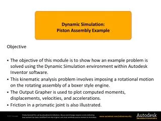
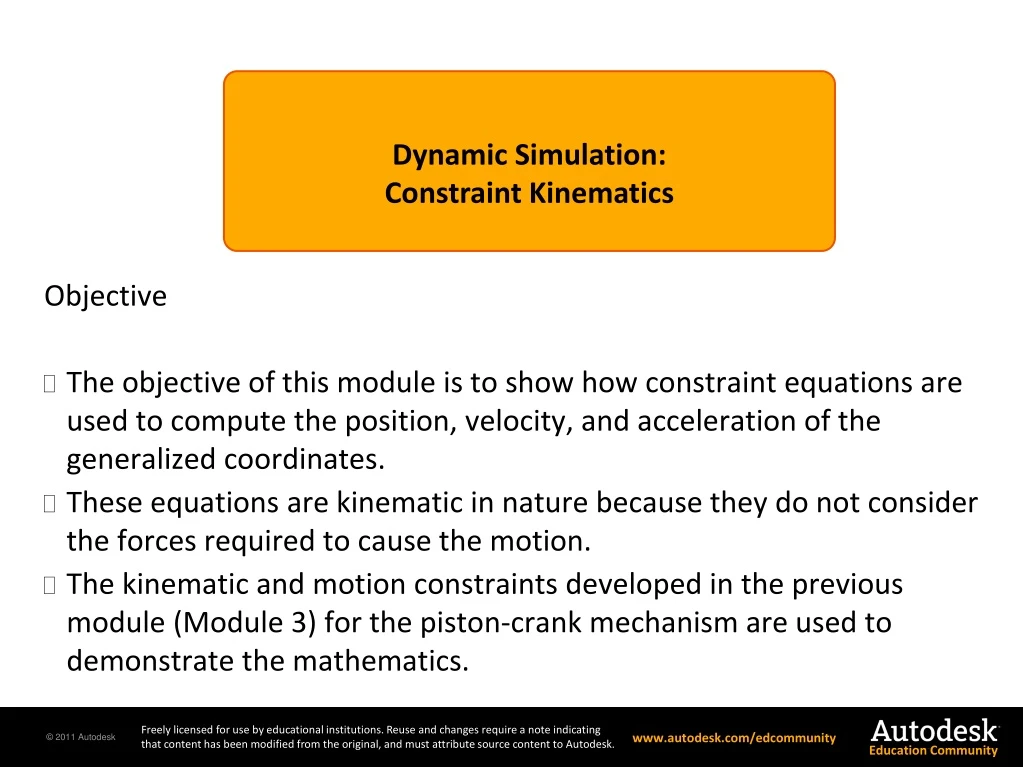
Dynamic Simulation : Constraint Kinematics. Objective The objective of this module is to show how constraint equations are used to compute the position, velocity, and acceleration of the generalized coordinates .

E N D
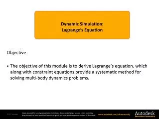
Dynamic Simulation: • Constraint Kinematics Objective • The objective of this module is to show how constraint equations are used to compute the position, velocity, and acceleration of the generalized coordinates. • These equations are kinematic in nature because they do not consider the forces required to cause the motion. • The kinematic and motion constraints developed in the previous module (Module 3) for the piston-crank mechanism are used to demonstrate the mathematics.
Section 4 – Dynamic Simulation Module 4 – Constraint Kinematics Page 2 • The total set of constraint equations needed to define a mechanism includes both kinematic constraints and drive constraints. • There are 15 generalized coordinates and 15 nonlinear constraint equations for the piston-crank assembly used in Module 3. • Since the piston-crank has a mobility of one, only one of the fifteen equations will be a motion constraint that is an explicit function of time. Notation is the set of generalized coordinates is the set of kinematic constraint equations is the set of motion constraint equations
Position Section 4 – Dynamic Simulation Module 4 – Constraint Kinematics Page 3 • Solving the constraint equations will yield the value of each generalized coordinate at a specific instance of time. • The constraint equations are non-linear and the Newton-Raphson method is used as the solution method. • The Newton-Raphson method is iterative and converges when the constraint equations are satisfied. Constraint Equations Newton-Raphson Equations where is the Jacobian matrix
Section 4 – Dynamic Simulation Module 4 – Constraint Kinematics Page 4 • The time derivative of the constraint equations is used to determine the velocities of the generalized coordinates. • Since the generalized coordinates are a function of time and the constraint equations are a function of the generalized coordinates and time, the chain rule for partial differentiation must be used. Constraint Equations Velocity Time Derivative Velocities
Section 4 – Dynamic Simulation Module 4 – Constraint Kinematics Page 5 • The second time derivative of the constraint equations is used to determine the accelerations of the generalized coordinates. • Since the generalized coordinates are a function of time and the constraint equations are a function of the generalized coordinates and time, the chain rule for partial differentiation must be used. 1st Time Derivative of Constraint Equations 2nd Time Derivative of Constraint Equations Acceleration Accelerations
Section 4 – Dynamic Simulation Module 4 – Constraint Kinematics Page 6 Constraint Equations Newton-RaphsonEquations Used to determine the position (values of the generalized coordinates) at an instant in time. Summary of Equations Velocities of Generalized Coordinates Accelerations of Generalized Coordinates
Jacobian Section 4 – Dynamic Simulation Module 4 – Constraint Kinematics Page 7 • The Jacobianand its inverse is needed to determine the position, velocity, and acceleration of the generalized coordinates. • Each i,j (row,column) term in the Jacobian matrix is given by Jacobian matrix Error messages indicating that the Jacobian is singular are sometimes encountered when running multi-body dynamic programs. This occurs when there is not a physically realizable solution. ith constraint equation jth generalized coordinate
Section 4 – Dynamic Simulation Module 4 – Constraint Kinematics Page 8 • The fifteen constraint equations developed for the piston-crank mechanism in Module 3 are given on the right. • Note that only the motion constraint is an explicit function of time. Piston-Crank Constraint Equations
Piston-Crank Jacobian Section 4 – Dynamic Simulation Module 4 – Constraint Kinematics Page 9 The Jacobian of the constraint equations is given below. Although there are many terms, there are a lot of zeros and the derivatives are easily computed.
Section 4 – Dynamic Simulation Module 4 – Constraint Kinematics Page 10 Motion Constraint • The velocities of the generalized coordinates are computed from the equation • Since the Jacobian is known, this equation can be solved if the array containing the time derivatives of the constraint equations is found. • Only the motion constraint, F(15), is an explicit function of time. Velocities Required Array
Section 4 – Dynamic Simulation Module 4 – Constraint Kinematics Page 11 The accelerations can be computed if each term is found. Acceleration This term is explained on the next slide. The time derivative of the Jacobian is zero. Inverse of the Jacobian
Acceleration Term Section 4 – Dynamic Simulation Module 4 – Constraint Kinematics Page 12 This term is evaluated by breaking it down into a series of operations that are easily done on a computer. Step 1) Multiply the Jacobian by the velocities. This creates a column array. Step 2) Take the derivative of each row with respect to each generalized coordinate. This operation is similar to finding the Jacobianand results in a matrix. Step 3) Multiply the matrix by the velocities. This results in a column array.
Redundant Constraints Section 4 – Dynamic Simulation Module 4 – Constraint Kinematics Page 13 • The rank of a matrix is equal to the number of independent rows or columns. • Independent rows or columns can not be written as a linear combination of other rows or columns. • If rows or columns of the Jacobian are not independent the Jacobian is singular and the problem does not have a solution. • The Jacobian matrix is an important quantity and enables the position, velocity, and acceleration of the generalized coordinates to be found. • Application of the methods contained in this module requires that the Jacobian have an inverse. • This requires that the determinant of the Jacobian be non-zero or that the rank be equal to the number of generalized coordinates.
Redundant Constraints: Detection Section 4 – Dynamic Simulation Module 4 – Constraint Kinematics Page 14 • The Dynamic Simulation environment within Autodesk Inventor software assembles the Jacobian and determines its rank as each constraint is added. • The rank gives the number of independent constraints. • The difference between the number of generalized coordinates and the number of independent constraints is equal to the degree of mobility. • The difference between the number of constraints and the number of independent constraints is equal to the degree of redundancy. nq number of generalized coordinates nc number of constraints nic number of independent constraints Degree of Mobility dom= nq – nic Degree of Redundancy dor = nc-nic
Redundant Constraints: Reaction Forces Section 4 – Dynamic Simulation Module 4 – Constraint Kinematics Page 15 • A redundant constraint occurs when the motion associated with a DOF is enforced by too many constraint specifications. • One or more of the constraint specifications can be removed without affecting the mobility of the system. • The joint reactions can not be independently determined when redundant constraints are present. • Although solutions can be obtained they are based on assumptions by the program as to which constraints to use. • Different assumptions will yield different answers. Joints having friction are particularly effected by redundant constraints. Friction forces are based on the joint normal forces. Therefore, the friction forces are incorrect if the joint normal forces are incorrect due to redundant constraints.
Redundant Constraint: Example Section 4 – Dynamic Simulation Module 4 – Constraint Kinematics Page 16 3 • A simple four bar mechanism will have redundant constraints if revolute joints are used at all joints. • The ground link shown in the figure is fixed. • The revolute joint at 1 prevents the drive link from rotating about its long axis and moving normal to the joint plane. • The revolute joint at 2 prevents the coupler from rotating about its long axis and moving normal to the joint plane. • The revolute joint at 4 prevents the rocker from rotating about its long axis and moving normal to the joint plane. Coupler Rocker 2 Drive 4 1 Ground A revolute joint at 3 is redundant because neither the rocker or coupler can rotate about their long axis or move normal to the joint plane due to the other revolute joints. These degrees of freedom are already restrained.
Redundant Constraints: Example Section 4 – Dynamic Simulation Module 4 – Constraint Kinematics Page 17 • A point-line joint must be used at joint 3. • A point-line joint restricts a point (the center point of the hole at joint 3 on the coupler) to remain on a line (the centerline of the hole at joint 3 on the rocker). • Redundant joints can be confusing and a detailed analysis of what each joint is doing is required to figure out how to remove them. • An example of how to remove redundant constraints is provided in the next module: Module 5. Point - Line 3 Coupler Revolute Rocker 2 Drive 4 1 Ground Revolute Revolute
Module Summary Section 4 – Dynamic Simulation Module 4 – Constraint Kinematics Page 18 • This module showed how the constraint equations can be used to find the position, velocity, and acceleration of the generalized coordinates. • Kinematic relationships were used during the derivation and no mention of the forces required to impose the motion constraints was made. • The constraint equations for the piston-crank introduced in the previous module (Module 3) were used to demonstrate the mathematical steps. • The Newton-Raphson method is generally used to solve the constraint equations. • The Jacobian is a key component of the overall solution process and the rank of the Jacobian is used to detect redundant constraints.