Download
1 / 30
300 likes | 409 Views
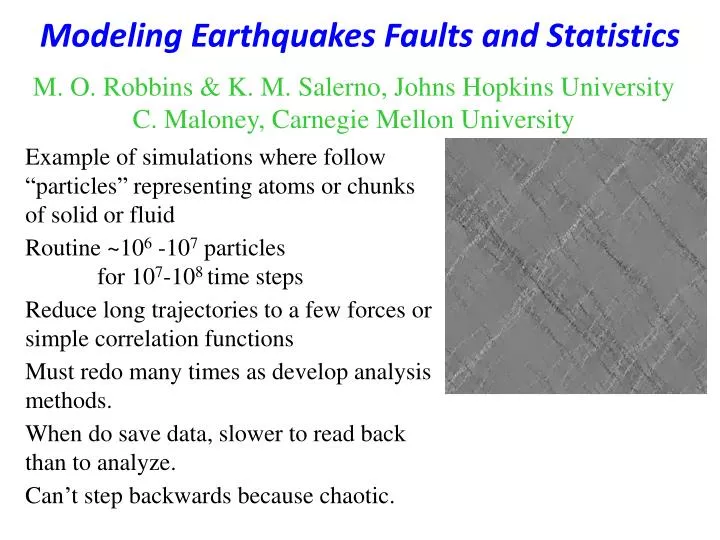
Modeling Earthquakes Faults and Statistics. M. O. Robbins & K. M. Salerno, Johns Hopkins University C. Maloney, Carnegie Mellon University. Example of simulations where follow “particles†representing atoms or chunks of solid or fluid

E N D
Modeling Earthquakes Faults and Statistics M. O. Robbins & K. M. Salerno, Johns Hopkins UniversityC. Maloney, Carnegie Mellon University Example of simulations where follow “particles” representing atoms or chunks of solid or fluid Routine ~106 -107 particles for 107-108 time steps Reduce long trajectories to a few forces or simple correlation functions Must redo many times as develop analysis methods. When do save data, slower to read back than to analyze. Can’t step backwards because chaotic.
Modeling Earthquakes Faults and Statistics M. O. Robbins & K. M. Salerno, Johns Hopkins UniversityC. Maloney, Carnegie Mellon University How do microscopic displacements accommodate total global strain? How are “earthquakes” distributed in energy, location and time? What is geometry of fault and nature of sliding on rough faults? Traditional approaches: Posit planar crack and follow dynamics Use actual structure, but assume no stress
Compression axis Motivation Vertical compression axis Textbook picture of brittle rock failure (from C. Scholz: The Mechanics of Earthquakes and Faulting) \ \ • Experiment: Uniaxial compression of rock • Otsuki and Dilov JGR 2005 • Scale ~ 20 cm situation of interest
Using atoms to model formation, evolution of strike-slip faults C.E. Maloney and M.O. Robbins Johns Hopkins and KITP Computing: UCSB CNSI
Push-ups Tensile fissures Motivation • Surface trace of earthquake in Iceland • Scale ~ 1km • From C. Scholz From C. Scholz: The Mechanics of Earthquakes and Faulting
Motivation • San Andreas Fault Network • Scale ~ 1000 km SCEC inter-seismic velocity map (displacement since 1984)
Method • Usually 2D Molecular Dynamics: • Binary Lennard-Jones Mean diameter s • Quenched at pressure p=0 • Relative velocity damping (Kelvin/DPD) • Periodic boundaries • Axial, fixed area strain or simple shear • Quasi-static limit, Controlled by Dg not Dt • Make system brittle by making all initial bonds 4 times stronger Prescribed Ly(t), Lx(t) to conserve area Ly(t) Lx(t)
Nonaffine Particle Displacements Non-affine displacement u = deviation from mean motion Integrate affine displacement along trajectory rather than using value for initial position. For each particle at each time step find distance moved relative to affine displacement at instantaneous position. Eliminates terms analogous to Taylor diffusion in simple shear Ly(t) Lx(t)
ω<0 ω>0 Local rotation, ω=u Find Delaunay triangulation for initial particle centers For each triangle: Invariants: “Left Strain” “Right Strain”
Mechanism for brittleness Brittle model: α=4. New bonds 4 times weaker. Ductile model: α=1. No “broken” bonds. Brittle 140 particles starts to fail patterns form Brittle Stress Ductile Strain Ductile
Pressure Induced Ductility Low pressure more brittle High pressure Stress Low pressure Strain High pressure more ductile
Total Shear Strain Incremental shear 10x10mm AFM image of clay “Earthquakes” in Large Brittle Systems
starts to fail patterns form Brittle Stress Ductile Strain Shift to Study of Ductile Systems Steady state strain accommodation
Spatial Variation of Nonaffine Displacement u Components of u during 0.2% strain+s white, -s black Strain localizes in plastic bands → step in total displacement uy ux Largest projection of u along bands ±45ºSign → rotation senseLength up to systemTypical a ~ s (ux+uy)/√2 (ux-uy)/√2
Displacement and w in steady state → Most analysis looks at magnitude Dr=| u | → smallest in plastic bandCurl sharply localized in plastic zone, +/- regions correlate along -/+45ºStrain accumulates to a~s in plastic bands through many avalanches →Displacement ~s allows all regions to find new metastable state Strain over intervals Dg > ~s/L occurs in uncorrelated locations |Dr| h~L/20 ω Strain g: 6.0% to 6.1% 6.0% to 6.2% 6.0% to 6.4%
Displacements Diffusive with DL Plastic band formed in each strain~a/L gives |Dr|<a/2, add incoherentlyDr2~Dg/(a/L) a2/12 ~ D Dg→ D ~ L a/12Consistent with observed D=57s2 for a=0.7s and for L down to 40 For w, no L dependence D=57s2
Distribution of Vorticity w Sharp elastic peak at small wExponential tails at large wWeight in tails grows ~linearly with strain Characteristic w* for decay ~0.1 Since w ~ twice strain, w* → 5% strain ~ yield strain Plastic bands have ~10 sharper localized bands
Vorticity Correlation Function Mean of log S scales as power of wave vector. Prefactor linear in Dg→Incoherent addition of successive intervals BUT scaling highly anisotropic
Angle Dependence of Structure Factor, Δγ=0.1% θ=π/8 θ=3π/8 θ=π/8 and θ=3π/8 have same shear stress, different normal stress. Mohr-Coulomb predicts shift to p/8 Α: broken shear symmetry bigger for planes with low normal loadas predicted by Mohr-Coulomb S(q;θ)=A(θ)q-α(θ) α = a+b cos(4q) A = c+d cos(2q)
Angle Dependence of Structure Factor, Δγ=0.1% θ=π/8 θ=3π/8 θ=π/8 and θ=3π/8 have same shear stress, different normal stress. Mohr-Coulomb predicts shift to p/8 Α: broken shear symmetry bigger for planes with low normal loadas predicted by Mohr-Coulomb S(q;θ)=A(θ)q-α(θ) α = a+b cos(4q) A = c+d cos(2q)
Gutenberg-Richter Law • Empirically determined scaling between earthquake number and magnitude • log(N) = C – bM • M = log(E) • Magnitude is the log of the energy released • Combined gives power law scaling: • Experimentally verified across regions, magnitude range b ~ 1
Avalanche Distribution ׀ Deformation through series of avalanches Find energy dissipated = change in potential energy - work done by system. Drops have wide distribution, 0.03 to 20 here Identify by sharp rises in dissipation rate. Dissipation rate/Kinetic energy drops to constant as energy moves to longest wavelengths. Ratio measures wavelength where have kinetic energy
P(E) = Number of Events per Unit Strain per E Reduce strain rate so quasi-static, only affects small events.Find power law P(E)~1/E over 5 decades.P(E) and maximum E increase with system size P(E)
Scaling Collapse of N(E) and E Scale E by Emax ~ Lb . Find b~1.1N(E/Emax) must scale as L1-b to maintain energy balance N(E) (L/100)1-b E*(L/100)2-b
Comparison to Scaling of P(E) in Other Models Same system but with energy minimization, not dynamics Exponent ~0.5 for largest systems Largest size ~3 Overdamped 2D Discrete dislocation model N(E)~E-tt=1.8 M.-C. Miguel, A. Vespignani, S. Zapperi, J. Weiss, and J.-R. Grasso, Mater. Sci. Eng., A 309–310, 324 2001. Why is power law different than Gutenberg-Richter? 3D amorphous metal N(E)~Exp[-E/Lx] x=1.4 N. P. Bailey, J. Schiøtz, A. Lemaître, and K. W. Jacobsen, PRL 98, 095501 (2007).
Our Quakes Include Fore and After ShocksHow Does this Affect Statistics?
Integrated Density of Quakes Based on Kinetic Energy Large events are broken up. Find integrated density ~ 1/E0.4
Conclusions • Strain localizes in plastic bands that extend across systemTypical slip distance along band a~particle diameterTypical thickness h scales with system size ~L/20Several sharper features in h with strain ~5 – 10% • Non-affine displacement Dr2~Dg/(a/L) a2/12 ~ D Dg, D~La/12 • Strain over short intervals has anisotropic power law correlationsS(|q|,q) ~ A(q) |q|-a(q) where α = a+b cos(4q), A = c+d cos(2q)Breaking of symmetry for A → Mohr-Coulomb • Inertial motion seems to lead to qualitative changes in deformation statistics. • Earthquake probability P(E) ~ 1/E over ~ 5 decadesExponent independent of geometry, interactionsMay depend on how events are broken up