Download
1 / 20
200 likes | 397 Views
Image reconstruction and Image Priors. Tim Rudge Simon Arridge, Vadim Soloviev Josias Elisee, Christos Panagiotou Petri Hiltunen (Helsinki University of Technology). Fast reconstruction algorithm Edge-based image priors Joint entropy image priors Gaussian-mixture classification priors.

E N D
Image reconstruction and Image Priors Tim Rudge Simon Arridge, Vadim Soloviev Josias Elisee, Christos Panagiotou Petri Hiltunen (Helsinki University of Technology)
Fast reconstruction algorithm • Edge-based image priors • Joint entropy image priors • Gaussian-mixture classification priors
1. Fast reconstruction • Image compression method • Reduce matrix size • Explicit fast inversion • Optics Letters, Vol. 35, Issue 5, pp. 763-765 (2010)
Forward operator • Size of matrix A = (nx* ny* ns* nθ) x nrecon = very big
i,j = source, detector • w = pixel detector profile • P = projection to image • S = diag(1/ye) = normalisation • Gf / Gf* = Green's operator / adjoint operator (fluorescent λ) • Ue = excitation field
Compress each image • Where rows of Z: ...are basis functions in image • E.g. Wavelets, Fourier (sine/cosine)
Form compressed system By replacing window functions w, with basis functions z in: Size of matrix = (nz* ns* nθ) x nrecon = more reasonable
Solve compressed system • Matrix is (nz* ns * nθ) x (nz* ns * nθ) • Small enough to store and solve explicitly • Typically solves in < 10s
2. Edge priors Smoothing operator Spatially varying width Edge in prior image low smoothing Smoothing max. ║ to edge Prior image flat max. Smoothing No segmentation needed
4. Gaussian-mixture priors Tikhonov 0 == single Gaussian Use mixture of k Gaussians Iteratively: K-means cluster class statistics Construct inv. covariance Cx-1, mean μx Reconstruct with prior Cx-1, μx
Combined Reconstruction Classification y Cy Data Noise Statistics x Reconstruction Step Estimation Step Image x,Cx l,q Class Statistics Image Statistics Prior Update Step
People / papers • Petri Hiltunen (Helsinki) – Gaussian-mixture priors • Phys. Med. Biol. 54, pp. 6457–6476, (2009) • Christos Panagiotou – Joint entropy priors • J. Opt. Soc. Am., Vol. 26, Issue 5, pp. 1277-1290, (2009) • Wavelet method: • Optics Letters, Vol. 35, Issue 5, (2010) pp. 763-765, (2010) • Martin Schweiger • TOAST FEM code, other programming • Josias Elisee • BEM method • Vadim Soloviev, Thanasis Zaccharopolous, Simon Arridge