Download
1 / 20
200 likes | 349 Views
Design and testing of a MOC monitoring array in the South Atlantic. Renellys C. Perez 12 , Silvia L. Garzoli 2 , Ricardo P. Matano 3 , Christopher S. Meinen 2 1 UM/CIMAS, 2 NOAA/AOML, 3 OSU/COAS. Existing and proposed observations in the South Atlantic.

E N D
Design and testing of a MOC monitoring array in the South Atlantic Renellys C. Perez12, Silvia L. Garzoli2, Ricardo P. Matano3, Christopher S. Meinen2 1UM/CIMAS, 2NOAA/AOML, 3OSU/COAS
Existing and proposed observations in the South Atlantic • International effort to constrain flow in/out of South Atlantic • Boundaries of box coincide with AX18, AX22, AX25 XBT lines • Nominal latitude of the northern boundary is 34.5°S Figure obtained from http://www.aoml.noaa.gov/phod/SAMOC/
South Atlantic MOC (SAM) array • Pilot array deployed in March 2009 along 34.5°S (3 PIES/1 CPIES) PIES (CPIES) = inverted echo sounder with bottom pressure sensor (and current meter) As part of BONUS-GOODHOPE project 2 CPIES were deployed near South African coast in February 2008 (Chief Scientist: Sabrina Speich) Figure from SAM Cruise report (Chief Scientist: Chris Meinen)
Objectives • Use models to determine optimal latitudes to monitor the MOC and northward heat transport (NHT) in the South Atlantic • Test whether a PIES/CPIES array can be used to monitor the MOC • Evaluate whether the SAM and Bonus-Goodhope arrays can be incorporated into a MOC monitoring array
Array development • Deploy virtual arrays into two high-resolution ocean models • Evaluate the ability of the arrays to reproduce the MOC and NHT • Perfect array of T, S profiles • Perfect array of CPIES* • SAM array + Bonus-Goodhope array (+ additional) • At each time step, velocity estimated as vg + vb + ve+ vc • Velocity adjusted by vc to give zero net volume transport • MOC(t) = maximum northward volume transport at each time step (integrate from velocity surface to ~1000 m) • Three-month low-pass filter applied to all time series • Focus on five latitudes: 15°S, 20°S, 25°S, 30°S, 34.5°S * IES travel times are combined with model T, S to produce time series of dynamic height and geostrophic velocity (similar to Gravest Empirical Mode methodology, e.g., Meinen et al. 2006)
Models • POCM: Parallel Ocean Circulation Model (Tokmakian and Challenor 1999) • Bryan (1969) primitive equation, hydrostatic, z-level model • ECMWF/ERA40 reanalysis fluxes • Horizontal resolution is 0.4° longitude x 1/4° latitude* • 20 z-levels • OFES: OGCM For the Earth Simulator (JAMSTEC) • Based on MOM3 • NCEP/NCAR reanalysis fluxes • Horizontal resolution is 0.1° longitude x 0.1° latitude • 54 z-levels 1Matano & Beier (2003),Schouten & Matano (2006),Baringer & Garzoli (2007),Fetter & Matano (2008) 2Sasaki et al. (2007), Giarolla & Matano (Ocean Sciences 2010)
MOC computed using perfect v array“Truth” Black = OFES Blue = POCM Left: MOC time series Right: Mean vertical structure
MOC computed using perfect v array“Truth” Lumpkin and Speer (2007) 11°S 16.2 ± 3.0 Sv 32°S 12.4 ± 2.6 Sv Dong et al. (2009) 35°S 17.9 ± 2.2 Sv
NHT computed using perfect v array“Truth” Black = OFES Blue = POCM Left: NHT time series Right: Mean vertical structure Correlation between NHT and MOC exceeds 0.85 for all latitudes and ΔQ/ΔV ~ 0.05 PW/Sv (similar to Dong et al. 2009)
Can a perfect T,S or CPIES array reconstruct the MOC in OFES? Black = “Truth” array Blue = Perfect T,S array Red = Perfect CPIES array Left: MOC time series Right: Mean vertical structure
Can a perfect T,S or CPIES array reconstruct the MOC in OFES? Less than 0.4 Sv bias at all latitudes High RMSE at 15°S Perfect T, S: high correlation at all latitudes Perfect CPIES: high correlation at 20°S, 30°S, 35°S
Can a perfect T,S or CPIES array reconstruct the MOC in POCM? Black = “Truth” array Blue = Perfect T,S array Red = Perfect CPIES array Left: MOC time series Right: Mean vertical structure
Can a perfect T,S or CPIES array reconstruct the MOC in POCM? Bias exceeds 1 Sv at low latitudes High RMSE at low latitudes Perfect T, S: high correlation at all latitudes Perfect CPIES: high correlation at 25°S, 30°S, 35°S
Summary • In general, better reconstructions are achieved • in OFES compared with POCM • at higher latitudes compared with lower latitudes • with a perfect T, S array compared with a perfect CPIES array • NHT is strongly correlated with the MOC • Higher latitudes better for placement of the SAMOC array, especially if array consists of PIES/CPIES • Preliminary modeling results from SAMOC3 meeting (May 11-13, 2010) suggest that nominal latitude of 35°S would be optimal for SAMOC array
OFES 34.5°S Blue = Degraded T,S array Red = Degraded CPIES array
Preliminary analysis shows that • Present arrays + 2 interior points perform surprisingly well at reproducing the MOC signal • The energetic Agulhas eddy region must be treated carefully • CPIES array and T, S array are comparable for MOC reconstructions • Need ~15 measurements to reproduce mean vertical structure of the MOC and have low biases
Future work • A more careful characterization of flow in bottom triangles is needed that better reflects the processing applied to RAPID/MOCHA data • SAMOC modeling community will work in close collaboration to simulate possible mooring configurations at nominal latitude of 34.5°S • Include additional ocean models/reanalyses • Synchronize our methodologies
POCM 34.5°S Blue = Degraded T,S array Red = Degraded CPIES array