Download
1 / 39
390 likes | 515 Views
Robotic Control. Lecture 1 Dynamics and Modeling. A brief history…. Started as a work of fiction Czech playwright Karel Capek coined the term robot in his play Rossum’s Universal Robots. Numerical control. Developed after WWII and were designed to perform specific tasks

E N D
Robotic Control Lecture 1 Dynamics and Modeling
A brief history… • Started as a work of fiction • Czech playwright Karel Capek coined the term robot in his play Rossum’s Universal Robots Robotic Control
Numerical control • Developed after WWII and were designed to perform specific tasks • Instruction were given to machines in the form of numeric codes (NC systems) • Typically open-loop systems, relied on skill of programmers to avoid crashes Robotic Control
Modern robots Mechanics Digital Computation Coordination Electronic Sensors Actuation Path Planning Learning/Adaptation Robotics Robotic Control
Types of Robots • Industrial • Locomotion/Exploration • Medical • Home/Entertainment Robotic Control
Industrial Robots Coating/Painting Assembly of an automobile Robotic Control Drilling/ Welding/Cutting
Locomotion/Exploration Underwater exploration Space Exploration Robo-Cop Robotic Control
Medical a) World's first CE-marked medical robot for head surgery b) Surgical robot used in spine surgery, redundant manual guidance. c) Autoclavable instrument guidance (4 DoF) for milling, drilling, endoscope guidance and biopsy applications Robotic Control
House-hold/Entertainment Toys Asimo Robotic Control
Purpose of Robotic Control • Direct control of forces or displacements of a manipulator • Path planning and navigation (mobile robots) • Compensate for robot’s dynamic properties (inertia, damping, etc.) • Avoid internal/external obstacles Robotic Control
Mathematical Modeling • Local vs. Global coordinates • Translate from joint angles to end position • Jacobian • coordinate transforms • linearization • Kinematics • Dynamics Robotic Control
Mechanics of Multi-link arms • Local vs. Global coordinates • Coordinate Transforms • Jacobians • Kinematics Robotic Control
Local vs. Global Coordinates • Local coordinates • Describe joint angles or extension • Simple and intuitive description for each link • Global Coordinates • Typically describe the end effector / manipulator’s position and angle in space • “output” coordinates required for control of force or displacement Robotic Control
Coordinate Transformation Cntd. • Homogeneous transformation • Matrix of partial derivatives • Transforms joint angles (q) into manipulator coordinates Robotic Control
Coordinate Transformation • 2-link arm, relative coordinates • Step 1: Define x and y in terms of θ1 and θ2 Robotic Control
Coordinate Transformation • Step 2: Take partial derivatives to find J Robotic Control
Joint Singularities • Singularity condition • Loss of 1 or more DOF • J becomes singular • Occurs at: • Boundaries of workspace • Critical points (for multi-link arms Robotic Control
Finding the Dynamic Model of a Robotic System • Dynamics • Lagrange Method • Equations of Motion • MATLAB Simulation Robotic Control
Step 1: Identify Model Mechanics Example: 2-link robotic arm Source: Peter R. Kraus, 2-link arm dynamics Robotic Control
Step 2: Identify Parameters • For each link, find or calculate • Mass, mi • Length, li • Center of gravity, lCi • Moment of Inertia, ii m1 i1=m1l12 / 3 Robotic Control
Step 3: Formulate Lagrangian • Lagrangian L defined as difference between kinetic and potential energy: • L is a scalar function of q and dq/dt • L requires only first derivatives in time Robotic Control
Kinetic and Potential Energies • Kinetic energy of individual links in an n-link arm • Potential energy of individual links Height of link end Robotic Control
Energy Sums (2-Link Arm) • T = sum of kinetic energies: • V = sum of potential energies: Robotic Control
Step 4: Equations of Motion • Calculate partial derivatives of L wrt qi, dqi/dt and plug into general equation: Non-conservative Forces (damping, inputs) Inertia (d2qi/dt2) Conservative Forces Robotic Control
Equations of Motion – Structure • M – Inertia Matrix • Positive Definite • Configuration dependent • Non-linear terms: sin(θ), cos(θ) • C – Coriolis forces • Non-linear terms: sin(θ), cos(θ), (dθ/dt)2, (dθ/dt)*θ • Fg – Gravitational forces • Non-linear terms: sin(θ), cos(θ) Robotic Control Source: Peter R. Kraus, 2-link arm dynamics
Equations of Motion for 2-Link Arm, Relative coordinates M- Inertia matrix Conservative forces (gravity) Coriolis forces, c(θi,dθi/dt) Robotic Control Source: Peter R. Kraus, 2-link arm dynamics
Alternate Form: Absolute Joint Angles • If relative coordinates are written as θ1’,θ2’, substitute θ1=θ1’ and θ2=θ2’+θ1’ • Advantages: • M matrix is now symmetric • Cross-coupling of eliminated from C, from F matrices • Simpler equations (easier to check/solve) Robotic Control
Matlab Code function xdot= robot_2link_abs(t,x) global T %parameters g = 9.8; m = [10, 10]; l = [2, 1];%segment lengths l1, l2 lc =[1, 0.5]; %distance from center i = [m(1)*l(1)^2/3, m(2)*l(2)^2/3]; %moments of inertia i1, i2, need to validate coef's c=[100,100]; xdot = zeros(4,1); %matix equations M= [m(2)*lc(1)^2+m(2)*l(1)^2+i(1), m(2)*l(1)*lc(2)^2*cos(x(1)-x(2)); m(2)*l(1)*lc(2)*cos(x(1)-x(2)),+m(2)*lc(2)^2+i(2)]; C= [-m(2)*l(1)*lc(2)*sin(x(1)-x(2))*x(4)^2; -m(2)*l(1)*lc(2)*sin(x(1)-x(2))*x(3)^2]; Fg= [(m(1)*lc(1)+m(2)*l(1))*g*cos(x(1)); m(2)*g*lc(2)*cos(x(2))]; T =[0;0]; % input torque vector tau =T+[-x(3)*c(1);-x(4)*c(2)]; %input torques, xdot(1:2,1)=x(3:4); xdot(3:4,1)= M\(tau-Fg-C); Robotic Control
Matlab Code t0=0;tf=20; x0=[pi/2 0 0 0]; [t,x] = ode45('robot_2link_abs',[t0 tf],x0); figure(1) plot(t,x(:,1:2)) Title ('Robotic Arm Simulation for x0=[pi/2 0 0 0]and T=[sin(t);0] ') legend('\theta_1','\theta_2') Robotic Control
Open Loop Model Validation Zero State/Input • Arm falls down and settles in that position Robotic Control
Open Loop - Static Equilibrium x0= [-pi/2 pi/2 0 0] x0= [-pi/2 –pi/2 0 0] x0= [pi/2 pi/2 0 0] x0= [pi/2 -pi/2 0 0] • Arm does not change its position- Behavior is as expected Robotic Control
Open Loop - Step Response Torque applied to second joint Torque applied to first joint • When torque is applied to the first joint, second joint falls down • When torque is applied to the second joint, first joint falls down Robotic Control
Input (torque) as Sine function Torque applied to first joint Torque applied to first joint • When torque is applied to the first joint, the first joint oscillates and the second follows it with a delay • When torque is applied to the second joint, the second joint oscillates and the first follows it with a delay Robotic Control
Robotic Control • Path Generation • Displacement Control • Force Control • Hybrid Control Robotic Control
Path Generation • To find desired joint space trajectory qd(t) given the desired Cartesian trajectory using inverse kinematics • Given workspace or Cartesian trajectory in the (x, y) plane which is a function of time t. • Arm control, angles θ1, θ2, • Convenient to convert the specified Cartesian trajectory (x(t), y(t)) into a joint space trajectory (θ1(t), θ2(t)) Robotic Control
Trajectory Control Types • Displacement Control • Control the displacement i.e. angles or positioning in space • Robot Manipulators • Adequate performance rigid body • Only require desired trajectory movement • Examples: • Moving Payloads • Painting Objects Robotic Control
Trajectory Control Types (cont.) • Force Control – Robotic Manipulator • Rigid “stiff” body makes if difficult • Control the force being applied by the manipulator – set-point control • Examples: • Grinding • Sanding Robotic Control
Trajectory Control Types (cont.) • Hybrid Control – Robot Manipulator • Control the force and position of the manipulator • Force Control, set-point control where end effector/ manipulator position and desired force is constant. • Idea is to decouple the position and force control problems into subtasks via a task space formulation. • Example: • Writing on a chalk board Robotic Control
Next Time… • Path Generation • Displacement (Position) Control • Force Control • Hybrid Control i.e. Force/Position • Feedback Linearization • Adaptive Control • Neural Network Control • 2DOF Example Robotic Control