Download

1 / 40
400 likes | 482 Views
Mobile Robotic Navigation Control in Moving Obstacle Environment. Rahul Kala, Department of Information Technology Indian Institute of Information Technology and Management Gwalior http://students.iiitm.ac.in/~ipg_200545/ rahulkalaiiitm@yahoo.co.in, rkala@students.iiitm.ac.in.

E N D
Mobile Robotic Navigation Control in Moving Obstacle Environment Rahul Kala, Department of Information Technology Indian Institute of Information Technology and Management Gwalior http://students.iiitm.ac.in/~ipg_200545/ rahulkalaiiitm@yahoo.co.in, rkala@students.iiitm.ac.in Paper: Kala, Rahul, et al (2009), Mobile Robot Navigation Control in Moving Obstacle Environment using Genetic Algorithm, Artificial Neural Networks and A* Algorithm, Proceedings of the IEEE World Congress on Computer Science and Information Engineering (CSIE 2009), ieeexplore, DOI 10.1109/CSIE.2009.854, pp 705-713, April 2009, Los Angeles/Anaheim, USA (Conference) (Download Paper)
Algorithms • A* Algorithm • Genetic Algorithm • Artificial Neural Networks
The Problem • There is a region of static and dynamic obstacles • Guide the robot from source o destination
Assumptions • The entire region divided in grid on size M X N • Each dynamic element can move not more than a unit distance in threshold time
Robotic Assumptions Various directions the robot can move in The representation of various directions
Robotic Assumptions The robotic movements • Move forward (unit step) • Move at an angle of 45 degrees forward (unit step) from the current direction • Move clockwise/anti-clockwise (45 degrees) • Move clockwise/anti-clockwise (90 degrees)
Robotic Movements Various Movements Possible
Costs • g(n) = depth from the initial node, increases by 1 in every step • h(n) = square of the distance of the current position and the final position + R(n) • R(n) = minimum time required for the robot to rotate in its entire journey assuming no obstacles • f(n) = g(n)+h(n)
3 2 Goal Position 1 4 R(n) The values of R(n) at various places Region 1: 0 Region 2: 2 Region 3: 1 Region 4: 1
NavigationPlan() Step 1: while(CurrentPosition <> FinalPosition) Begin Step 2: m ← getNextRobotMove(CurrentPosition) Step 3: moveRobot(m)
getNextMove(CurrentPosition) Step 1: closed ← empty list Step 2: add a node n in open such that position(n) = CurrentPosition Step 3: while open is not empty Begin Step 4: extract the node n from open with the least priority Step 5: if n = final position then break Step 6: else Step 7: moves ← all possible moves from the position n Step 8: for each move m in moves Begin Step 9: if m leads us to a point which can be the point of any obstacle in the next unit time then discard move m and continue Step 10 if m is already in open list and is equally good or better then discard this move Step 11: if m is already in closed list and is equally good or better then discard this move Step 12 delete m from open and closed lists Step 13: make m as new node with parent n Step 14: Add node m to open Step 15: Add n to closed Step 16: Remove n from open
0(N) 2(E) 3(SE) 1(NE) 4(S) 5(SW) 6(W) 7(NW) Testing The representation of obstacles in various directions
Genetic Algorithm • We consider a graphical representation of chromosome • Each chromosome a collection of graphical nodes • Crossover operation by graph mixing
Types Of solutions • Full: They are complete solution and fully connect source to destination • Left: The start from the source but are unable to reach to the destination • Right: They do not start from the source but reach the destination
Types Of solutions Full Left Left Right Right
Fitness Function • Full Solution: f(S)=No of steps needed to traverse from source to destination • Left Solution: Number of steps needed to traverse from source to the last point traversed + (Square of the distance of this point to the final destination + R(n)) • Right Solution: (Square of the distance of source point to the first point traversed + R(n)) + Number of steps needed to traverse from this point to the final solution
Initial Solution • Try to find a straight path solution between source and destination • Try to find random left solution between source and destination • Try to find random right solution between source and destination. • Find Full Solutions from fusion of left and right
Initial Solution Step1: for i ← 1 to noIterationsInitial Begin Step2: for j ← 1 to (3/2)*perimeter of board (Maximum moves per solution being tried) Begin Step3: if p ← destinationPoint Step4: add p to current solution set and break Step5: find the move m in moves which makes the robot closest to destination Step6: if point p we reach after m is already in the current solution set then delete earlier points and add this point. Step7: if no move takes the robot closer to target Step 8: make randomMoves number of random moves in any direction Step9: for each move m in these moves, if point p we reach after m is already in the current solution set then delete earlier points and add this point. Step10: if destinationPoint is reached then add this solution set to fullSolution Step11: else add this solution set to leftSolution
Crossover • The crossover can occur between any of the following pairs of solutions • Full Solution and Full Solution • Left Solution and Full Solution • Full Solution and Right Solution • Left Solution and Right solution
CrossOver(parent1,parent2) Step 1: points ← find common points in parent1 and parent2 that have same x and y coordinate Step 2: if points <> null Step 3: for each common point p in points Begin Step4: sol1 ← all points in parent1 till p + rotations necessary to transform direction of p to the one of point p of parent2 + all points in parent2 after p Step5: Add sol1 to fullSolution set
Mutate Step 1: if no of solutions in full solution set > 0 then Step 2: r1,r2 ← any two random points on a random solution from fullSolution set set with r1 on the left of r2 Step 3: find solutions as found in initial solution with start point as r1 and goal point as r2 Step 4: if full results generated > 0 Step 5: newSolution ← most fit solution in this generated solution set Step 7: sol1 ← all points in solution till r1 + rotations necessary to transform direction of r1 to the one of first point of newSolution + all points in newSolution + rotations necessary to transform direction of last point in newSolution to r2 + all points in solution after r2 Step 8: add sol1 to solutionFull
Selection • With a probability of 2/3, select the most fit chromosome from the full solution set and any one randomly from the left/right/full solution set • With a probability 1/3 select any random chromosome from full solution set and any one randomly from left/right/full solution set
Inputs There are total 26 inputs to the neural network (I0-I25) • The I0 and I1 denote the rotations • (I0,I1)=(0 0) represents +2 or -2 • (I0,I1)=(0 1) represents +1 • (I0,I1)=(1 1) represents 0 • (I0,I1)=(1 0) represents -1 These are numbered according to gray codes
Outputs • 3 Outputs (O0,O1,O2)=(0,0,0) Rotate left 90 degrees. (O0,O1,O2)=(0,0,1) Rotate left 45 degrees. (O0,O1,O2)=(0,1,0) Move forward. (O0,O1,O2)=(0,1,1) Rotate left 45 degrees and move forward. (O0,O1,O2)=(1,0,0) Do not move. (O0,O1,O2)=(1,0,1) Rotate right 90 degrees. (O0,O1,O2)=(1,1,0) Rotate right 45 degrees and move forward. (O0,O1,O2)=(1,1,1) Move right 45 degrees.
GenerateTestCases() Step 1: initialize map and generate N obstacles at positions (xi,yi,di) Step 2: while(noTestCaseGenerated <> noTestCasesDesired) Begin Step 3: Generate the robot at random position (xi,yi,di) Step 4: I ← Input sequence Step 5: m ← getNextRobotMoveUsingAStar(CurrentPosition) Step 6: moveRobot(m) Step7: O ← Output Sequence Step 8: Add (I,O) to training data
NavigationPlan() Step 1: n ← Generate Neural Network Step 2: n ← TrainNeuralNetwork() Step 3: while(CurrentPosition <> FinalPosition) Begin Step 4: I ← generateInputSequence() Step 5: O ← generateOutputSequence(I) Step6: if O gives valid move Step 7: moveRobot(O) Step 8: if robot not changed position in last 5 steps Step 9: makeRandomMove() Step10: if distance of robot decreasing in last 5 steps (excluding rotations) Step11: move next move only if the next move decreases distance or is of equal distance