Download
1 / 42
420 likes | 552 Views
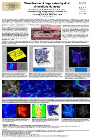
Visualization. Visualization. Parallel Visualization of Large-Scale Datasets for the Earth Simulator. Li Chen Issei Fujishiro Kengo Nakajima. Basic Design & Parallel/SMP/Vector Algorithm. Research Organization for Information Science and Technology (RIST) Japan.

E N D
Visualization Visualization Parallel Visualization of Large-Scale Datasets for the Earth Simulator Li Chen Issei Fujishiro Kengo Nakajima Basic Design & Parallel/SMP/Vector Algorithm Research Organization for Information Science and Technology (RIST) Japan 3rd ACES Workshop, May 5-10, 2002, Maui, Hawaii.
Background Role of Visualization Subsystem Earth Simulator Hardware Software GeoFEM Application analysis Vis Subsys Solver Mesh gen. Tools for: (1) Post Processing (2) Data Mining etc.
Background: Requirements Target 1: Powerful visualization functions Translate data from numerical forms to visual forms. Provide the researchers with immense assistance in the process of understanding their computational results. We have developed many visualization techniques in GeoFEM, for scalar, vector and tensor data fields, to reveal data distribution from many aspects. Target 2: Suitable for large-scale datasets High parallel performance Our modules have been parallelized and obtained a high parallel performance Target 3: Available for unstructured datasets Complicated grids All of our modules are based on unstructured datasets, and can be extended to hybrid grids. Target 4: SMP cluster architecture oriented Three-level hybrid parallelprogramming model is adopted in our modules Effective based on the SMP cluster architecture
Works after 2nd ACES (Oct. 2000) • Developed more visualization techniques for GeoFEM • Improved parallel performance • Please Visit Our Poster for Detail !!
Overview • Visualization Subsystem in GeoFEM • Newly Developed Parallel Volume Rendering (PVR) • Algorithm • Parallel/Vector Efficiency • Examples • Future Works
Visualization Result Files Visualization Result Files FEM Analysis Mesh Files FEM-#0 mesh #0 result #0 VIS-#0 I/O Solver I/O UCD etc. FEM-#1 mesh #1 result #1 VIEWER AVS etc. VIS-#1 Images I/O Solver I/O Input Output Communication FEM-#n-1 mesh #n-1 result #n-1 VIS-#n-1 I/O Solver I/O Parallel VisualizationFile Version or “DEBUGGING” Version on Client includes simplification, combination etc.
Huge Large-Scale Data in GeoFEM 1km x 1km x 1km mesh for 1000km x 1000km x 100km "local" region 1000 x 1000 x 100 = 108 grid points 1GB/variable/time step ~10GB/time step for 10 variables TB scale for 100 steps !!
Visualization Result Files Mesh Files FEM+Visualization on GeoFEM Platform mesh #0 FEM-#0 VIS-#0 I/O Solver I/O UCD etc. mesh #1 FEM-#1 VIS-#1 VIEWER AVS etc. Images I/O Solver I/O on Client Input Output Communication mesh #n-1 VIS-#n-1 FEM-#n-1 I/O Solver I/O Parallel VisualizationMemory/Concurrent Version Dangerous if detailed physics is not clear
Parallel Visualization Techniques in GeoFEM Scalar Field Vector Field Tensor Field Cross-sectioning Streamlines Hyperstreamlines Isosurface-fitting Particle Tracking Surface-fitting Topological Map Interval Volume-fitting LIC Volume Rendering Volume Rendering In the following, we will take the Parallel Volume Rendering module as example to demonstrate our strategies on improving parallel performance available June 2002, http://geofem.tokyo.rist.or.jp/
Visualization Subsystem in GeoFEM • Newly Developed Parallel Volume Rendering (PVR) • Algorithm • Parallel/Vector Efficiency • Examples • Future Works
Design of Visualization Methods Principle Taking account of parallel performance Taking account of huge data size Taking account of unstructured grids Classification of Current Volume Rendering Methods Grid type Regular Curvilinear Traversal Approach Image-order volume rendering (Ray casting) Object-order volume rendering (Cell projection) Unstructured Hybrid order volume rendering Composition Approach Projection Parallel From front to back Perspective From back to front
Design of Visualization Methods Principle Taking account of concurrent with computational process Classification of Parallelism Object-space parallelism Partition object space and each PE gets a portion of the dataset. Each PE calculates an image of the sub-volume. Image-space parallelism Partition image space and each PE calculates a portion of the whole image. Time-space parallelism Partition time space and each PE calculates the images of several timesteps.
Design for Parallel Volume Rendering Unstructured Locally Refined Octree/Hierarchical Why not unstructured grid? • Hard to build hierarchical structure • Connectivity information should be found beforehand • Unstructured grid makes image composition and load balance difficult • Irregular shape makes sampling slower regular grid? Why not • Large storage requirement • Slow down volume rendering process
Parallel Transformation PE#0 PE#1 PE#2 PE#3 PE#4 PE#5 PE#6 PE#7 PE#8 PE#9 PE#10 PE#11 PE#12 PE#13 PE#14 PE#15 PE#16 PE#17 Voxels Background Cells Original GeoFEM Meshes Unstructured Hierarchical One Solution Ray-casting PVR Resampling VR Image Hierarchical data FEM Data
Accelerated Ray-casting PVR Build Branch-on-need octree Hierarchicaldatasets Determine sampling and mapping parameters VR parameters Generate subimages for each PE for each subvolume for j=startj to endj do for i=starti to endi do Fast find the intersection voxels with ray (i,j) Compute (r,g,b) at each intersection voxel based on volume illumination model and transfer functions Compute (r,g,b) for pixel(i,j) based on front-to-back composition Build topological structure of subvolumes on all PEs Composite subimages from front to back
Visualization Subsystem in GeoFEM • Newly Developed Parallel Volume Rendering (PVR) • Algorithm • Parallel/Vector Efficiency • Examples • Future Works
Memory Memory Memory Memory Memory P E P E P E P E P E P E P E P E P E P E P E P E P E P E P E P E P E P E P E P E SMP Cluster Type Architectures • Earth Simulator • ASCI Hardwares • Various Types of Communication, Parallelism. • Inter-SMP node, Intra-SMP node, Individual PE
Optimum Programming Modelsfor Earth Simulator ? Each PE Intra NODE Inter NODE F90 + directive(OpenMP) MPI F90 MPI HPF MPI HPF Memory P E P E P E
Three-Level Hybrid parallelization Flat MPI parallelization Each PE: independent Hybrid Parallel Programming Model Based on Memory hierarchy • Inter-SMP node MPI • Intra-SMP node OpenMP for parallelization • Individual PE Compiler directives for vectorization/pseudo vectorization
Memory Memory P E P E P E P E P E P E P E P E Flat MPI vs. OpenMP/MPI Hybrid Memory Memory P E P E P E P E P E P E P E P E Flat-MPI:Each PE -> Independent Hybrid:Hierarchal Structure
Three-Level Hybrid parallelization Previous work on hybrid parallelization R. Falgout, and J. Jones, "Multigrid on Massively Parallel Architectures", 1999. F. Cappelo, and D. Etiemble, "MPI versus MPI+OpenMP on the IBM SP for the NAS Benchmarks", 2000. K. Nakajima and H. Okuda, "Parallel Iterative Solvers for Unstructured Grids using Directive/MPI Hybrid Programming Model for GeoFEM Platform on SMP Cluster Architectures", 2001 All these are in computational research area. No visualization papers are found on this topic. Previous parallel visualization methods Classification by platform •Shared memory machines: J. Nieh and M. Levoy 1992, P. Lacroute 1996 •Distributed memory machines: U. Neumann 1993, C. M. Wittenbrink and A. K. Somani, 1997 • SMP cluster machines: almost no papers are found.
SMP Cluster Architecture Node-0 Node-1 PE M e m o r y PE M e m o r y PE PE PE PE Node-0 Node-1 PE PE PE PE PE PE PE PE PE PE Node-2 Node-3 PE M e m o r y PE M e m o r y PE PE PE PE PE PE PE PE PE PE PE PE Partitioning of data domain PE PE Node-2 Node-3 The Earth Simulator 640 SMP nodes, and 8 vector processors in each SMP node
Three-Level Hybrid parallelization Criteria to achieve high parallel performance • Local operation and no global dependency • Continuous memory access • Sufficiently long loops
Vectorization for Each PE Construct Vectorizatoin Loop •Combine some short loops into one long loop by reordering for(i=0;i<MAX_N_VERTEX; i++) for(j=0;j<3;j++) { p[i][j]=…. …. } for(i=0;i<MAX_N_VERTEX*3; i++){ p[i/3][i % 3]=…. …. } •Exchange the innermost and outer loop to make the innermost loop longer for(j=0;j<3;j++) for(i=0;i<MAX_N_VERTEX; i++){ p[i][j]=…. …. } for(i=0;i<MAX_N_VERTEX; i++) for(j=0;j<3;j++) { p[i][j]=…. …. } •Avoid using tree and single/double link data structure, especially in the inner loop link (single or double) structure tree structure
3 4 3 4 3 4 3 4 1 2 1 2 1 2 1 2 3 4 3 4 3 4 3 4 1 2 1 2 1 2 1 2 Intra-SMP Node Parallelization OpenMP http://www.openmp.org Multi-coloring for Removing the Data Race [Nakajima, et al. 2001] Ex: gradient computation in PVR #pragma omp parallel { for(i=0;i<num_element;i++) { compute jacobian matrix of shape function; for(j=0; j<8;j++) { for(k=0; k<8;k++) accumulate gradient value of vertex j contributed by vertex k; } } } PE#0 PE#1 PE#2 PE#3
Inter-SMP Node Parallelization MPI Parallel Data Structure in GeoFEM External node Internal node Communication Overlapped elements are used for reducing communication among SMP nodes Overlap removal is necessary for final results
Dynamic Load Repartition Why? Rendered voxels often accumulate in small portions of the field during visualization Initial partition on each PE: (Same with analysis computing) almost equal number of voxels Load on each PE: (PVR process) the number of rendered voxels Load balance during PVR Keep almost equal number of rendered voxels on each PE Number of non-empty voxels Opacity transfer functions Viewpoint Dynamic
Dynamic Load Repartition Most previous methods Scattered decomposition[K.-L. Ma, et al, 1997] • Advantage: Can get very good load balance easily • Disadvantage Large amount of intermediate results have to be stored • Large extra memory • Large extra communication Assign several continuous subvolumes on each PE • Count the number of rendered voxels during the process of gird transformation • Move a subvolume from a PE with a larger number of rendered voxels to another PE with a smaller one
Dynamic Load Repartition Assign several continuous subvolumes on each PE • Count the number of rendered voxels during the process of gird transformation • Move a subvolume from a PE with a larger number of rendered voxels to another PE with a smaller one PE1 PE0 PE1 PE0 PE2 PE3 PE3 PE2 Initial partition Repartition
Visualization Subsystem in GeoFEM • Newly Developed Parallel Volume Rendering (PVR) • Algorithm • Parallel/Vector Efficiency • Examples • Future Works
Speedup Test 1 Demonstrate the effect of three-level hybrid parallelization Dataset: Pin Grid Array (PGA) dataset (Data courtesy of H. Okuda and S. Ezure). Simulate the Mises Stress distribution on the pin grid board by the Linear Elastostatic Analysis Data size: 7,869,771 nodes and 7,649,024 elements Running environment SR8000 Each node: 8 PEs 8GFLOPS peak performance 8GB memory Total system: 128 nodes (1024 PEs) 1.0TFLOPS peak performance 1.0TB memory
Speedup Test 1 Top view Bottom view Volume rendered images to show the equivalent scalar value of stress by the linear elastostatic analysis for a PGA dataset with 7,869,771 nodes and 7,649,024 elements (Data courtesy of H. Okuda and S. Ezure).
Speedup Test 1 Comparison of speedup performance between flat MPI and the hybrid parallel method for our parallel volume rendering module. Original (MPI) to Vector Version (Hybrid) Speed-up for 1PE : 4.30 1283 Uniform Cubes for PVR
Speedup Test 2 Demonstrate the effect of three-level hybrid parallelization Test Dataset: Core dataset (Data courtesy of H. Matsui in GeoFEM) Simulate thermal convection in a rotating spherical shell Data size: 257,414 nodes and 253,440 elements Test Module Parallel Surface Rendering module Running environment SR8000 Each node: 8 PEs 8GFLOPS peak performance 8GB memory Total system: 128 nodes (1024 PEs) 1.0TFLOPS peak performance 1.0TB memory
Speedup Test 2 Pressure isosurfaces and temperature cross-sections for a core dataset with 257,414 nodes and 253,440 elements. The speedup of our 3-level parallel method is 231.7 for 8 nodes (64PEs) on SR8000.
Speedup Test 2 Comparison of speedup performance between flat MPI and the hybrid parallel method for our parallel surface rendering module. Original (MPI) to Vector Version (Hybrid) Speed-up for 1PE : 4.00
Speedup Test 3 Demonstrate the effect of dynamic load repartition Dataset: Underground water dataset Simulate groundwater flow and convection/diffusion transportation through heterogeneous porous media 200100100 Region Different Water Conductivity for 16,000, 128,000, 1,024,000 Meshes (∆h= 5.00/2.50/1.25) 100 timesteps Running environment Compaq alpha 21164 cluster machine (8 PEs, 600MHz/PE, 512M RAM/PE) Result For mesh 3 (about 10 million cubes and 100 timesteps) Without dynamic load repartition: 8.15 seconds for one time-step averagely. After dynamic load repartition: 3.37 seconds for one time-step averagely.
Speedup Test 3 Groundwater Flow Channel Dh= 5.00 Dh=2.50 Dh=1.25 Effects of convection & diffusion for different mesh sizes
Application (2) • Flow/Transportation • 505050 Region • Different Water Conductivity for each (Dh=5)3 cube • df/dx=0.01, f=0@xmax • 1003 Meshes • Dh= 0.50 • 64PEs : Hitachi SR2201
Parallel PerformanceConvection & Diffusion • 13,280 steps for 200 Time Unit • 106 Meshes, 1,030,301 Nodes • 3,984 sec. for elapsed time including communication on Hitachi SR2201/64PEs • 3,934 sec. for real CPU • 98.7% parallel performance
Convection & DiffusionVisualization by PVR Groundwater Flow Channel
Conclusions and Future Work Improve Parallel Performance of Visualization Subsystem in GeoFEM ● Improve the parallel performance of the visualization algorithms ● Three-level hybrid parallel based on SMP cluster architecture • Inter-SMP node MPI • Intra-SMP node OpenMP for parallelization • Individual PE Compiler directives for vectorization/pseudo vectorization ● Dynamic load balancing Future Work Tests on the Earth Simulator http://www.es.jamstec.go.jp/