Download
1 / 22
220 likes | 325 Views
The Architecture of Earth Simulator. Gülfem IŞIKLAR 09.12.2004. Introduction Supercomputers Vector Processing The Earth Simulator Conclusion. Outline. Introduction. Image Processing. Testing Car Crashes. Medical Diagnosis. C reating N ew C hemical S ubstances.

E N D
The Architecture of Earth Simulator Gülfem IŞIKLAR 09.12.2004
Introduction Supercomputers Vector Processing The Earth Simulator Conclusion Outline
Introduction Image Processing Testing Car Crashes Medical Diagnosis Creating New Chemical Substances More Powerful Computers Climate Changes Gene Technology Space Exploration Global Warming Effects
Supercomputer :A computer that is able to operate at a speed that places it at or near the top speed of currently produced computers. The first supercomputers were introduced in the 1960s, designed primarily by Seymour Crayat Control Data Corporation (CDC). Supercomputers
On November 2004, according to the TOP500, the first 5 supercomputers are : 1. BlueGene/L, Doe/IBM, USA with perf : 70.72 TFLOPS 2. Columbia, NASA/Ames, USA with perf : 51.87 TFLOPS 3. Earth Simulator, Earth Simulator Center, Yokohama with perf : 35.86 TFLOPS 4. MareNostrum, Barcelona Supercomputer Center, Spain with perf : 20.53 TFLOPS 5. Thunder, Lawrence Livermore National Lab, USA with perf : 19.94 TFLOPS Supercomputers
Vector Processing : A program roughly takes the form of applying the same computation to a big chunk of data. Vector computers have instructions which can operate on strings of numbers formed as one-dimensional arrays (vectors). One operation can be specfied on all elements of vector in a single instruction. Basically, vector processing is a version of the Single Instruction Multiple Data (SIMD) parallel processing technique. Vector Processing
The main point: A single vector instruction represents a lot of basic scalar operations.
The computation of each result (in vector processor) is independent of the computation of previous results. A single vector instruction specifies a great deal of work - it is equivalent to executing an entire loop. Vector instructions that access memory have a known access pattern. If the vector's elements are all adjacent, then fetching the vector from a set of heavily interleaved memory banks works very well. Vector Processing Properties
Conventional Computer Initialize I = 0 20 Read B(I) Read C(I) Store A(I) = B(I) + C(I) Increment I = i + 1 If I 100 goto 20 1. A vector of values in B(I) will be fetched from memory. 2. A vector of values in C(I) will be fetched from memory. 3. A vector add instruction will operate on pairs of B(I) and C(I) values. 4. Stream of A(I) values will be stored back to memory, one value every clock cycle. Vector Programming
Vector Computer A(1:100) = B(1:100) + C(1:100) 1. B(1) will be fetched from memory. 2. C(1) will be fetched from memory. 3. A scalar add instruction will operate on B(1) and C(1). 4. A(1) will be stored back to memory 5. Step (1) to (4) will be repeated 100 times. Vector Programming
The machine has to fetch and decode far fewer instructions, so the control unit overhead is greatly reduced and the memory bandwidth necessary to perform this sequence of operations is reduced a corresponding amount. • The instruction provides the processor with a regular source of data. When the vector instruction is initiated, the machine knows it will have to fetch n pairs of operands which are arranged in a regular pattern in memory. With an interleaved memory, the pairs will arrive at a rate of one per cycle, at which point they can be routed directly to a pipelined data unit for processing. Vector Processing
Milestones of Development The Earth Simulator Initiation : In 1997, The Earth Simulator Research and Development Center has been established. Conceptual design :It has been proposed by NEC Corporation and has been selected by bidding. 2002: The ES has achieved the performance of 26.78 TFLOPS by using the atmospheric general circulation model (AFES) which was the highest performance record. November 2004: The ES is the third supercomputer in TOP500 list.
A vector architecture should be employed which is an efficient architecture for large-scale scientific simulations. • The system design should be as compact as possible in order to limit the space and electric power. As a result, the vector processor should be realized as a one-chip LSI. • The memory bandwidth achieved should be 128 TB/s in order to maintain the peak performance which is more than 32 TFLOPS/s. So, a distributed main memory system should be used. • A single-stage crossbar network should be taken in order to make the system completely homogeneous. • A multiple job environment should be provided at operation of the ES. Design Concepts
Each AP consist of 4-way superscalar unit, a vector unit, a main memory control unit on a single LSI chip. Each SU is a super-scalar processor with 64KB instruction cache, 64KB data cache, and 128 general-purpose scalar registers. Each VU has 72 vector registers, each of which has 256 vector elements, along with 8 sets of six different types of vector pipelines. The Arithmetic Processor (AP)
The Processor Nodes (NP) The 640 processor nodes are connected via a 640 x 640 single-stage crossbar switched.
The memory system in a PN is equally shared by 8 APs and is configured with 32 main memory units, each of which has one memory port and is interconnected with a crossbar switch. Each processor within a node can have access to 32 memory ports when vector load/store instruc-tions are issued. Each processor has a data transfer rate of 32 GB/s with memory devices, which results in the aggregate throughput of 256 GB/s per node. The Memory System
There are two important major application groups in the ES project: Conclusion • 1. High resolution atmospheric and oceanographic models which are global models to predict global warming and El Nino event, regional models to predict Asian Monsoon and typhoon, and local model to predict weather disasters such as torrential rain falls and downbursts. • 2. The applications in the field of solid earth science which are global models to describe longrange crustal movements, regional models to understand mechanism of seismicity and seismic wave propagation, and local models to understand migration of underground water and materials transfer in strata.
References [1] Earth Simulator Home Page, http://www.es.jamstec.go.jp/esc/eng/ES/ [2] M. Yokokawa, S. Shingu, S. Kawai, K. Tani, and H. Miyoshi (1998),Performance Estimation of the Earth Simulator, Proceedings of 8th ECMWF Workshop, World Scientific, 34-53. [3] Shingu S., Takahara H., Fuchigami H., Yamada M., Tsuda Y., Ohfuchi W., Sasaki Y., Kobayashi K., Hagiwara T., Habata S., Yokowawa M., Itoh H., Otsuka K. (2002),A 26.58 Tflops Global Atmospheric Simulation with the Spectral Transform Method on the Earth Simulator, IEEE. [4] Yokokawa M. (2001),Present Status of Development of the Earth Simulator, IEEE.