Download
1 / 12
130 likes | 276 Views
Ch4 Short-time Fourier Analysis of Speech Signal.

E N D
Ch4 Short-time Fourier Analysis of Speech Signal Fourier analysis is the spectrum analysis. It is an important method to analyze the speech signal. Short-time Fourier analysis is a stationary analytic method to process the non-stationary signal (speech signal). It is also called time dependent Fourier transformation.
4.1 Short-time Fourier Transformation (1) • 4.1.1 Definition of Short-time Fourier Transformation • Xn(ejω) = Σx(m)w(n-m) e-jωm where n is discrete and ωis continuous • It is calledshort-time Fourier transform function or time-frequency function • two interpretations: n = n0, it is a spectrum function; ω= ω0 , it is a output of bandpass filter w(n) whose center frequency is ω0 .
4.2 Spectrograms Based on Short-time Fourier Transformation(1) • 4.2.1 Frequency energy density function Pn(ω) • Pn(ω) = |X(expjω)|2 = ΣRn(k)exp(jωk) • Rn(k)= Σx(m)w(n-m)x(m+k)w(n-m-k) m=-∞~∞ • Note: if window length is L, Rn(k) has length 2L • If we make the picture according to Pn(ω) : • the x axis is time, the y axis is frequency, the pixel’s greygrade is Pn(ω), and the picture is called spectrogram (or sonogram).
Spectrograms Based on Short-time Fourier Transformation(2) • 4.2.2 Frequency resolution • According to previous interpretation, n is fixed. Xn(expjω) is the spectrum. x(n) times w(n) corresponds the convolution of X(ω) and W(ω). So the bandwidth of W(ω) b will affect the frequency resolution. If high frequency resolution is required, b should be small and N should large (b~1/N), that means window length should be large.
Spectrograms Based on Short-time Fourier Transformation(3) • 4.2.3 Time resolution • According to previous second interpretation, ω is fixed. The role of w(n) corresponds a low-pass filter for x(n) exp(jnωk). The bandwidth of output is the bandwidth of w(n) b. According to sampling theorem, sample rate is 2b. The time resolution is 1/(2b). If high time resolution is required, b should be large, and N should be small. These two resolutions are contradictory.
Spectrograms Based on Short-time Fourier Transformation(4) • 4.2.4 Sonogram of wide or narrow bands • For practical purpose sometime we need both. • Wide band has window length 6.4ms, narrow band 51.2ms (examples), a window with 1s length has 2Hz bandwidth. So the frequency resolution for two case are 39Hz(narrow) and 313Hz(wide). Wide for seeing formants. Narrow for seeing the change of pitch and structure of harmonic wave.
4.4Perceptually Motivated Representations (1) • 4.4.1 The Bark and Mel Scales • Fleccher’s work pointed to the existence of critical bands in the cochlear response. Critical bands are of great importance in understanding many auditory phenomena such as perception of loudness, pitch and timbre. The auditory system performs frequency analysis of sounds into their component frequencies. One class of critical band is called Bark frequency scale. It is hoped that by treating spectral energy over the Bark scale, a more natural fit with spectral information processing in the ear can be achieved. The Bark scale ranges from 1 to 24 Barks, corresponding to 24 critical bands of hearing :
Perceptually Motivated Representations (2) • Bark Band # Edge(Hz) Center(Hz) 1 100 50 2 200 150 3 300 250 4 400 350 5 510 450 6 630 570 7 770 700 8 920 840 9 1080 1000 10 1270 1170 11 1480 1370 12 1720 1600
Perceptually motivated Representations (3) • Bark Band # Edge(Hz) Center(Hz) 13 2000 1850 14 2320 2150 15 2700 2500 16 3150 2900 17 3700 3400 18 4400 4000 19 5300 4800 20 6400 5800 21 7700 7000 22 9500 8500 23 12000 10500 24 15500 13500
Perceptually Motivated Representations (4) • 4.4.2 Mel scale frequency cepstrum • Mel scale is another scale such that 1000Hz correspond to 1000 mels: Mel(f) = 1125ln(1+f/700) • How to get the MFCC : Xa[k] = Σn=0N-1x(n)e-j2nk/N S[m] = ln[Σk=0N-1|Xa[k]|2Hm(k)]
Perceptually Motivated Representations (5) Hm[k] is a triangle filter : 0 k<f[m-1] Hm[k]=2(k-f[m-1])/{(f[m+1]-f[m-1])(f[m]-f[m-1])} f[m-1]<=k<=f[m] 2(f[m+1]-k)/{(f[m+1]-f[m-1])(f[m+1]-f[m])} f[m]<=k<=f[m+1] 0 k>f[m+1]
Perceptually Motivated Representations (6) • c(n) = Σm=0N-1S[m]cos(n(m+1/2)/M) 0<=n<=M • M is 24-40. c(n) only take the first 12-13. • MFCC is extensively used in speech circle. • Besides MFCC themselves, the first order and second order of the differences of these coefficients are used as components of the feature vector. • dn(t)= Σj=1L j(cn[t+j]-cn[t-j]/(2Σj=1Lj2) n=1~12 • an(t)= Σj=1L j(dn[t+j]-dn[t-j]/(2Σj=1Lj2) n=1~12