Download
1 / 54
540 likes | 559 Views
Learn how to convert non-linear curves to linear form through variable transformations for enhanced analysis. Covers various transformation techniques with examples.

E N D
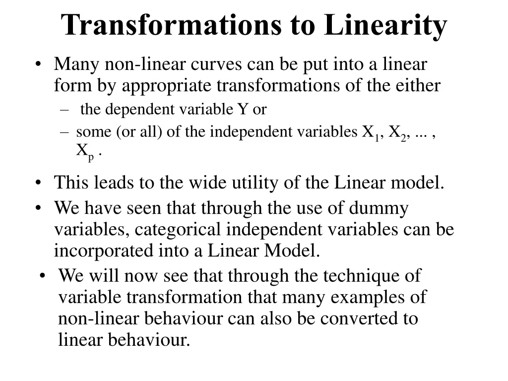
Transformations to Linearity • Many non-linear curves can be put into a linear form by appropriate transformations of the either • the dependent variable Y or • some (or all) of the independent variables X1, X2, ... , Xp . • This leads to the wide utility of the Linear model. • We have seen that through the use of dummy variables, categorical independent variables can be incorporated into a Linear Model. • We will now see that through the technique of variable transformation that many examples of non-linear behaviour can also be converted to linear behaviour.
Intrinsically Linear (Linearizable) Curves 1 Hyperbolas y = x/(ax-b) Linear form: 1/y = a -b (1/x) or Y = b0 + b1 X Transformations: Y = 1/y, X=1/x, b0 = a, b1 = -b
2. Exponential y = a ebx = aBx Linear form: ln y = lna + b x = lna + lnB x or Y = b0 + b1 X Transformations: Y = ln y, X = x, b0 = lna, b1 = b = lnB
3. Power Functions y = a xb Linear from: ln y = lna + blnx or Y = b0 + b1 X
Logarithmic Functions y = a + b lnx Linear from: y = a + b lnx or Y = b0 + b1 X Transformations: Y = y, X = ln x, b0 = a, b1 = b
Other special functions y = a eb/x Linear from: ln y = lna + b 1/x or Y = b0 + b1 X Transformations: Y = ln y, X = 1/x, b0 = lna, b1 = b
Polynomial Models y = b0 + b1x + b2x2 + b3x3 Linear form Y = b0 + b1 X1 + b2 X2 + b3 X3 Variables Y = y, X1 = x , X2 = x2, X3 = x3
Linear form lny = b0 + b1 X1 + b2 X2 + b3 X3+ b4 X4 Y = lny, X1 = x , X2 = x2, X3 = x3, X4 = x4 Exponential Models with a polynomial exponent
b0, d1, g1, … , dk, gk are parameters that have to be estimated, • n1, n2, n3, … , nk are known constants (the frequencies in the trig polynomial. Note:
Dependent variable Y and two independent variables x1 and x2. (These ideas are easily extended to more the two independent variables) Response Surface models The Model (A cubic response surface model) or Y = b0 + b1X1 +b2X2 + b3X3 +b4X4 + b5X5 + b6X6 + b7X7 + b8X8 + b9X9+ e where
y up y up x down x up x down x up y down y down The Bulging Rule
Non-Linear Growth models The Mechanistic Growth Model • many models cannot be transformed into a linear model Equation: or (ignoring e) “rate of increase in Y”=
The Logistic Growth Model Equation: or (ignoring e) “rate of increase in Y”=
The Gompertz Growth Model: Equation: or (ignoring e) “rate of increase in Y”=
Example: daily auto accidents in Saskatchewan to 1984 to 1992 Data collected: • Date • Number of Accidents Factors we want to consider: • Trend • Yearly Cyclical Effect • Day of the week effect • Holiday effects
Trend This will be modeled by a Linear function : Y = b0 +b1X (more generally a polynomial) Y = b0 +b1X +b2X2+ b3X3+ …. Yearly Cyclical Trend This will be modeled by a Trig Polynomial – Sin and Cos functions with differing frequencies(periods) : Y = d1 sin(2pf1X)+ g1 cos(2pf2X)+ d1 sin(2pf2X) + g2 cos(2pf2X) + …
Day of the week effect: This will be modeled using “dummy”variables : a1D1 + a2D2 + a3D3 + a4D4 + a5D5 + a6D6 (more generally a polynomial) Di = (1 if day of week = i, 0 otherwise) Holiday Effects Also will be modeled using “dummy”vaiables :
Independent variables X = day,D1,D2,D3,D4,D5,D6,S1,S2,S3,S4,S5, S6,C1,C2,C3,C4,C5,C6,NYE,HW,V1,V2,cd,T1, T2. Si=sin(0.017202423838959*i*day). Ci=cos(0.017202423838959*i*day). Dependent variable Y = daily accident frequency
Independent variables ANALYSIS OF VARIANCE SUM OF SQUARES DF MEAN SQUARE F RATIO REGRESSION 976292.38 18 54238.46 114.60 RESIDUAL 1547102.1 3269 473.2646 VARIABLES IN EQUATION FOR PACC . VARIABLES NOT IN EQUATION STD. ERROR STD REG F . PARTIAL F VARIABLE COEFFICIENT OF COEFF COEFF TOLERANCE TO REMOVE LEVEL. VARIABLE CORR. TOLERANCE TO ENTER LEVEL (Y-INTERCEPT 60.48909 ) . day 1 0.11107E-02 0.4017E-03 0.038 0.99005 7.64 1 . IACC 7 0.49837 0.78647 1079.91 0 D1 9 4.99945 1.4272 0.063 0.57785 12.27 1 . Dths 8 0.04788 0.93491 7.51 0 D2 10 9.86107 1.4200 0.124 0.58367 48.22 1 . S3 17 -0.02761 0.99511 2.49 1 D3 11 9.43565 1.4195 0.119 0.58311 44.19 1 . S5 19 -0.01625 0.99348 0.86 1 D4 12 13.84377 1.4195 0.175 0.58304 95.11 1 . S6 20 -0.00489 0.99539 0.08 1 D5 13 28.69194 1.4185 0.363 0.58284 409.11 1 . C6 26 -0.02856 0.98788 2.67 1 D6 14 21.63193 1.4202 0.273 0.58352 232.00 1 . V1 29 -0.01331 0.96168 0.58 1 S1 15 -7.89293 0.5413 -0.201 0.98285 212.65 1 . V2 30 -0.02555 0.96088 2.13 1 S2 16 -3.41996 0.5385 -0.087 0.99306 40.34 1 . cd 31 0.00555 0.97172 0.10 1 S4 18 -3.56763 0.5386 -0.091 0.99276 43.88 1 . T1 32 0.00000 0.00000 0.00 1 C1 21 15.40978 0.5384 0.393 0.99279 819.12 1 . C2 22 7.53336 0.5397 0.192 0.98816 194.85 1 . C3 23 -3.67034 0.5399 -0.094 0.98722 46.21 1 . C4 24 -1.40299 0.5392 -0.036 0.98999 6.77 1 . C5 25 -1.36866 0.5393 -0.035 0.98955 6.44 1 . NYE 27 32.46759 7.3664 0.061 0.97171 19.43 1 . HW 28 35.95494 7.3516 0.068 0.97565 23.92 1 . T2 33 -18.38942 7.4039 -0.035 0.96191 6.17 1 . ***** F LEVELS( 4.000, 3.900) OR TOLERANCE INSUFFICIENT FOR FURTHER STEPPING
Non-Linear Regression Introduction Previously we have fitted, by least squares, the General Linear model which were of the type: Y = b0 + b1X1 + b2 X2 + ... + bpXp + e
the above equation can represent a wide variety of relationships. • there are many situations in which a model of this form is not appropriate and too simple to represent the true relationship between the dependent (or response) variable Y and the independent (or predictor) variables X1 , X2 , ... and Xp. • When we are led to a model of nonlinear form, we would usually prefer to fit such a model whenever possible, rather than to fit an alternative, perhaps less realistic, linear model. • Any model which is not of the form given above will be called a nonlinear model.
This model will generally be of the form: Y = f(X1, X2, ..., Xp| q1, q2, ... , qq) + e * where the function (expression) f is known except for the q unknown parameters q1, q2, ... , qq.
Suppose that we have collected data on the Y, • (y1, y2, ...yn) • corresponding to n sets of values of the independent variables X1, X2, ... and Xp • (x11, x21, ..., xp1) , • (x12, x22, ..., xp2), • ... and • (x12, x22, ..., xp2).
For a set of possible values q1, q2, ... , qq of the parameters, a measure of how well these values fit the model described in equation * above is the residual sum of squares function • where • is the predicted value of the response variable yi from the values of the p independent variables x1i, x2i, ..., xpi using the model in equation * and the values of the parameters q1, q2, ... , qq.
The Least squares estimates of q1, q2, ... , qq, are values • which minimize S(q1, q2, ... , qq). • It can be shown that the error terms are independent normally distributed with mean 0 and common variance s2 than the least squares estimates are also the maximum likelihood estimate of q1, q2, ... , qq).
To find the least squares estimate we need to determine when all the derivatives S(q1, q2, ... , qq) with respect to each parameter q1, q2, ... and qq are equal to zero. • This quite often leads to a set of equations in q1, q2, ... and qq that are difficult to solve even with one parameter and a comparatively simple nonlinear model. • When more parameters are involved and the model is more complicated, the solution of the normal equations can be extremely difficult to obtain, and iterative methods must be employed.
To compound the difficulties it may happen that multiple solutions exist, corresponding to multiple stationary values of the function S(q1, q2, ... , qq). • When the model is linear, these equations form a set of linear equations in q1, q2, ... and qq which can be solved for the least squares estimates . • In addition the sum of squares function, S(q1, q2, ... , qq), is a quadratic function of the parameters and is constant on ellipsoidal surfaces centered at the least squares estimates .
Techniques for Estimating the Parameters of a Nonlinear System • In some nonlinear problems it is convenient to determine equations (the Normal Equations) for the least squares estimates , • the values that minimize the sum of squares function, S(q1, q2, ... , qq). • These equations are nonlinear and it is usually necessary to develop an iterative technique for solving them.
In addition to this approach there are several currently employed methods available for obtaining the parameter estimates by a routine computer calculation. • We shall mention three of these: • 1) Steepest descent, • 2) Linearization, and • 3) Marquardt's procedure.
In each case a iterative procedure is used to find the least squares estimators . • That is an initial estimates, ,for these values are determined. • The procedure than finds successfully better estimates, that hopefully converge to the least squares estimates,
Steepest Descent • The steepest descent method focuses on determining the values of q1, q2, ... , qq that minimize the sum of squares function, S(q1, q2, ... , qq). • The basic idea is to determine from an initial point, and the tangent plane to S(q1, q2, ... , qq) at this point, the vector along which the function S(q1, q2, ... , qq) will be decreasing at the fastest rate. • The method of steepest descent than moves from this initial point along the direction of steepest descent until the value of S(q1, q2, ... , qq) stops decreasing.
It uses this point, as the next approximation to the value that minimizes S(q1, q2, ... , qq). • The procedure than continues until the successive approximation arrive at a point where the sum of squares function, S(q1, q2, ... , qq) is minimized. • At that point, the tangent plane to S(q1, q2, ... , qq) will be horizontal and there will be no direction of steepest descent.
It should be pointed out that the technique of steepest descent is a technique of great value in experimental work for finding stationary values of response surfaces. • While, theoretically, the steepest descent method will converge, it may do so in practice with agonizing slowness after some rapid initial progress.
Slow convergence is particularly likely when the S(q1, q2, ... , qq) contours are attenuated and banana-shaped (as they often are in practice), and it happens when the path of steepest descent zigzags slowly up a narrow ridge, each iteration bringing only a slight reduction in S(q1, q2, ... , qq).
A further disadvantage of the steepest descent method is that it is not scale invariant. • The indicated direction of movement changes if the scales of the variables are changed, unless all are changed by the same factor. • The steepest descent method is, on the whole, slightly less favored than the linearization method (described later) but will work satisfactorily for many nonlinear problems, especially if modifications are made to the basic technique.
Steepest Descent Steepest descent path Initial guess
Linearization • The linearization (or Taylor series) method uses the results of linear least squares in a succession of stages. • Suppose the postulated model is of the form: Y = f(X1, X2, ..., Xp| q1, q2, ... , qq) + e • Let be initial values for the parameters q1, q2, ... , qq. • These initial values may be intelligent guesses or preliminary estimates based on whatever information are available.
These initial values will, hopefully, be improved upon in the successive iterations to be described below. • The linearization method approximates f(X1, X2, ..., Xp| q1, q2, ... , qq) with a linear function of q1, q2, ... , qq using a Taylor series expansion of f(X1, X2, ..., Xp| q1, q2, ... , qq) about the point and curtailing the expansion at the first derivatives. • The method then uses the results of linear least squares to find values, that provide the least squares fit of of this linear function to the data .
The procedure is then repeated again until the successive approximations converge to hopefully at the least squares estimates:
Linearization Contours of RSS for linear approximatin 2nd guess Initial guess