Download
1 / 89
910 likes | 946 Views
METEOROLOGICAL PARAMETERS FROM SATELLITE IMAGERY CLOUD MOTION VECTORS. WIND COVERAGE TRADITIONAL WEATHER BALLOONS. SATELLITE WINDS.

E N D
METEOROLOGICAL PARAMETERS FROM SATELLITE IMAGERY CLOUD MOTION VECTORS
SATELLITE WINDS The idea of using successive satellite observations of clouds to determine wind direction and speed was pioneered by Professor Suomi of the University of Wisconsin-Madison. While the concept is simple, the procedure is rather complex.
Satellite Derived Winds Cover the globe and are available at multiple levels
BASIC PRINCIPLE 40N/85E 38.5N/83.2E
BASIC PRINCIPLE 40N/85E 38.5N/83.2E
BASIC PRINCIPLE • A problem we have in tracking clouds is that we do not know the path they take • If we can determine the path they take we can determine the wind direction. • Watch the image of the car on the previous page and imagine that you did not have the roadway to help determine the car's path. • A good way to determine the path of the car is to track two images of the car that are close in time. • The same thinking applies to clouds. We view two images of a cloud that are close in time. Long time intervals are not good for tracking clouds that are changing rapidly. Short time intervals (1 to 15 minutes) are best when clouds are moving quickly.
Satellite Derived Winds • A sequence of Geo Stationery Sat images, separated by 15 or 30 minutes, are used to compute winds from satellite images. • This is particularly useful over the oceans where conventional weather observations are not possible. While it's true that buoys and ships send in weather observations they simply can't contribute anywhere near the coverage offered by satellites. • The accuracy of weather forecasts improved dramatically during the 1990's due to the addition of satellite derived winds in forecast models. This has been especially crucial to the timing and location of where a hurricane makes landfall.
Satellite Derived Winds The meteorological data on a global scale are so important for initialization purposes in Numerical Weather Prediction. Particularly over data-sparse areas like Indian Ocean, can be met only through derivation of products indirectly from satellite data. Satellites basically measure the radiance reaching them from the earth’s surface and cloud tops. By making such measurements in appropriate wavelengths applying physical and statistical techniques, it is possible to compute a wide range of products.
Some of the common parameters derived from the satellite images Atmospheric Motion Vectors (AMV) Outgoing Long wave Radiation(OLR) Quantitative Precipitation Estimates (QPE) Sea Surface Temperatures(SST)
Atmospheric Motion Winds (AMV) Cloud Motion Vectors ( CMV) Using Visible Band Using Infrared band 2. Water Vapour Winds (WVW) Using Water Vapour Band
Basic Concept Derivation of a Wind Vector from the motion of the clouds. As we know that frequent images of the same area are only possible from the geo-stationary satellites. Therefore, by tracking the movement of the same cloud in successive images can give a good estimate of the winds
Basic Concept As shown in the figure , a cloud in image at time T is positioned at A( i,j ) and same cloud is positioned at B( i,j) in image at time T + T, then“A vector difference of the location of a cloud in two successive images divided by the time interval between images is an estimate of the horizontal wind at the level of the cloud” The difference between the two successive images could be 30 min, 7.5 min or 3 min. The lesser value of difference can give more number of good quality winds.
Indian Geostationary Meteorological Satellites At present, there are three Indian Geostationary Meteorological Satellites.
INSAT-2E, INSAT-3AMeteorological Payload : (i) VHRR(ii) CCD (i) VHRR (ii) CCD
CLOUD MOTION VECTORS Cloud Motion Vectors are being derived both from Infrared and Visible data of Kalpana-1 & Insat-3A Satellites from the triplets of following imagery : Time in UTCCMV’s From 1) 23:30, 00:00, 00:30 IR Kalpana-1 • 07:00, 07:30, 08:00 IR, VIS Kalpana-1 • 11:30, 12:00, 12:30 IR Insat-3A • 18:00, 18:30, 19:00 IR Insat-3A
STEPS IN THE COMUTATION OF CMV’s • In general, there are five steps in the derivation of Cloud Motion Vectors : • Registration of Triplet • Cloud Tracers selection • Tracking of Cloud Tracer in Target image • CMV Computation • Height Assignment • Quality Control of Cloud
Registration of Images Registration implies that when two images are displayed in time sequence, the land features should look stationary. In other words, two images are said to be registered if the landmarks in one image exactly overlay on the other image. The registration is achieved by shifting one image with respect to the other till the landmarks are lined up in both the images.
In Insat Meteorological Data Processing System (IMDPS), every reception is navigated automatically as a part of near real time processing. If required, the capabilities (NAV-SHIFT) are applied which exercise the North-South or East-West translational shifts or rotation to achieve the accuracy of Navigation. It is presumed that frame to frame registration is achieved as result of accurate navigation and the computation of Vector Displacement uses latitude/longitude of the initial and final points of the Vector.
The steps of cloud tracer selection • Tracer Location List Generation • Tracer Threshold Calculation • Tracer Histogram Generation • Tracer Selection
FOUR BIN HISTOGRAM FORIR IMAGERY f r e q u e n c y LOW MEDIUM CLEAR HIGH 0 0 pixel intensities 255
Criteria For Tracer Selection At every selected location, a box of 16 x 16 pixels is considered, Total Number of pixel in a box = 256 From the Four-Bin Histogram Total Number of low cloud pixels = NcL Total Number of medium cloud pixels = Ncm Total Number of high cloud pixels = Nch Total Number of cloudy pixels = Nc NC = NCL + NCM + NCH contd. 16 16
Criteria For Tracer Selection If the number of clear pixels contained in a box is equal to or greater than 85 % of total pixels, the box is treated as CLEAR (N - NC) > 85% of N If the number of cloudy pixels contained in a box is equal to or greater than 90 % of total pixels, the box is treated as CLOUDY NC > 90% of N Out of NCL , NCM and NCH , whichever is highest , the tracer is identified to be of that type.
TRACKING THE CLOUD TRACERS There are two basic methods of tracking of clouds Manual Tracking Automatic Tracking
Manual Tracking In this technique, an analyst locates the clouds to be tracked on each of two successive images. This is generally done by positioning a cursor at the cloud on a video display device. Advantages Even low clouds can be tracked through thin cirrus overcast. Theoretically, more number of vectors can be obtained. Disadvantages It is tedious and limits the number of tracers
Automatic Tracking In this method, individual clouds cannot be tracked. A pattern of clouds are tracked. Therefore, the average motion of an area of clouds is calculated. The automatic tracking is done primarily using the Cross Correlation method.
TRACKING THE CLOUD TRACERS CMV’s are being derived from two pairs of three half-hourly images at 0000Z, 0730 Z , 1200Z & 1800Z TARGET IMAGE TARGET IMAGE TRACER IMAGE 00Z CMV’s FROM 2330 0030 0000Z 07:30Z CMV’s FROM 0800 0700 0730
TRACER IMAGE TARGET IMAGE Pattern Matching by Cross Correlation 16 16 (p,q) Best Fit Search Window (S) Reference Window (T) • Search window size for Low clouds is 36 • Search window size for Medium clouds is 44 • Search window size for High clouds is 52
Cross Correlation At each of the lag position (p,q), the cross correlation is calculated by the following formula N N (T(i,j) – T) (S(i+p, j+q) – S(p,q)) i = 1 j=1 C(p,q)= N N N N 2 2 (T(i,j) – T) (S(i+p, j+q)-S(p,q)) i=1 j=1 j=1 i=1 Where T is the array of pixel intensities from the reference window and T is the mean, and S is the array of sub-set of search window at lag position (p,q) and S is the mean at that position The lag position (p,q) where the correlation coefficient is maximum is assumed to be the final position of the vector
MASKING OPTION Cloud tracking becomes difficult if multi-layer clouds are present in the scene. To overcome this difficulty, IMDPS has a provision of ‘Masking Option’. All pixels in the reference and the Search window which were not identified as part of a specific cluster are masked out.
CLOUD MOTION VECTOR CALCULATION The CMV calculation is done in the following manner : (i) Target cloud classification / verification (ii) Vector Calculation
Target Cloud Classification/Verification This is basically a validation step so as to ensure that the same cloud pattern was tracked. For each of the tracked cloud targets, the four bin histogram is generated as was done for the cloud tracer and the same classification criteria is applied. The cloud target is rejected if it is not of the type of cloud tracer.
Vector Calculation The center of the reference / search window is the initial point of the vector and the location for which absolute maximum peak is obtained as the final position of the vector. From these positions, CMV is calculated. If correlation returns multiple locations with the same maximum value, the first one is accepted.
CMV Height Assignment Height assignment of the CMV’s is being done using Infrared Window (IRW) technique at present. Mean temperature of the 25% coldest IR pixels (John LeMarshal et al. 1993, Merrill R 1989, Nieman S. J et al. 1997) is considered for assigning the height of the CMV. The software of the system is being upgraded and the H2O- IRW Intercept Method will also be tried shortly.
Problems in Height Assignment Problems are due to semitransparent clouds (such as cirrus) or sub pixel clouds (small clouds not filling the sensor field of view) Since the fraction of the sensor field of view occupied by the cloud is less than unity by an unknown amount, the brightness temperature Tb in the IR window is usually an overestimate of the cloud temperature. Thus, heights for semitransparent or subpixel clouds inferred directly from the observed Tb and an available temperature profile is consistently low
Quality Control Regarding quality control of the generated cloud motion vectors, the general approach is as follows: : • Reasonable Minimum and Maximum Limits of CMV • Testing the spatial and temporal consistencies of the vectors • Comparison of the vectors with forecast field vectors • Comparison with climatology in the event of non-availability of forecast field
Absolute Threshold Test Speed Test Directional Stability Test Gradient Test Forecast Test Climatology Test Editing of Cloud Motion Vectors OBJECTIVE QUALITY CONTROL
Absolute Threshold Test The two vectors (VBA and VBC ) generated from two pairs of images are individually checked for the limits of speeds possible for various cloud types i.e. |VBA| and |VBc| > Min. Speed, and |VBA| and |VBc| < Max. Speed A B C Target image at time T + h Target image at time T - h Tracer image at time T 1 1 2 2 VBC VBA
Speed Test In order to ensure that the two speeds do not have a large difference, this test is applied. ||VBA| - | VBc | | < 0.5 Vaverage where Vaverage = | VBA | + | VBC | 2
Direction Stability Test This is basically to ensure temporal consistency. • If Vaverage < 20 Kts and the direction difference between VBA and VBc is more than 60, the CMV is rejected • If 60 > Vaverage > 20 and the direction difference between VBA and VBc is more than 40 , the CMV is rejected and • If Vaverage > 60 Kts and the direction difference between VBA and VBc is more than 20 , the CMV is rejected.
RESULTANT VECTOR At this stage, the average VB of the two vectors viz. VBA and VBC is computed through U and V components which is then subjected to following tests. • Gradient Test • Forecast Field Test • Climatological Test
GRADIENT TEST Basically , this is to testhorizontal consistency . • Speed difference between VB and the surrounding vectors must be less than the gradient speed threshold (20 kts). • Direction difference between VB and surrounding vectors must be less than the gradient direction threshold (45). • Distance from VB and the surrounding vectors must be less than the gradient distance threshold (300 Km.)
Forecast Field Test This is to test CMV’s against the forecast wind field produced by different centres of the world. At present, IMDPS CMV’s are being checked against the forecast field from Limited Area Model, IMD. • Speed difference between VB and the surrounding field must be less than 20 kts. • Direction difference between VB and the surrounding field must be less than 45 • Distance between VB and the surrounding field must be less than 300 Km.
Climatological Test If the forecast field is not available due to any reasons, the CMV’s are checked against climatology. The criteria of the test is same as that of forecast field.
Man-Machine Interactive Editing The CMV’s which have passed objective tests are available for interactive editing by the analyst at the work station. The CMV’s can be displayed on the monitor and the analyst can flag all those vectors which are inconsistent with the general field of motion. However, any deviant CMV can be retained if the cloud pattern suggest the likely existence of some new or rapidly changing circulation system. It is also possible to change the level of CMV.
Medium Level CMV’s Derived from Infrared of Kalpana-1 23-May-04
High Level CMV’s Derived from Infrared of Kalpana-1 23-May-04