Download
1 / 36
360 likes | 460 Views
Examining the impact of aerosol direct effects in the coupled WRF-CMAQv5.0 modeling system. K. Wyat Appel 11 th Annual CMAS Conference October 16, 2012. Acknowledgments. David Wong (Two-way code) Shawn Roselle Jon Pleim Rohit Mathur Christian Hogrefe (spectral density)

E N D
Examining the impact of aerosol direct effects in the coupled WRF-CMAQv5.0 modeling system K. Wyat Appel 11th Annual CMAS Conference October 16, 2012
Acknowledgments • David Wong (Two-way code) • Shawn Roselle • Jon Pleim • RohitMathur • Christian Hogrefe (spectral density) • Chao Wei (Two-way simulations)
Motivation • Conventional CMAQ air quality simulations utilize meteorological inputs that are run independently of the Chemical Transport Model (CTM) • The coupled WRF-CMAQ system runs the meteorological model and CTM together, which allows for communication (feedback) between the two models • feedback is important for including the effects that aerosols have on the meteorological fields (e.g. solar radiation) • more realistic representation of the atmosphere • In this work, the coupled WRF-CMAQ modeling system is used to: • examine impact of aerosol direct effects on model estimates (performing simulations with and without aerosol direct effects)
CMAQ Coupled Simulations CMAQv5.0 Modeling System - 12km CONUS AQMEII domain - CB05 chemistry - GEOS-Chem boundary conditions - lightning NO emissions included - wind-blown dust January and June 2006 - coupled w/ aerosol direct effects (F) - coupled w/o aerosol direct effects (NF) Coupled model simulations (w/ feedback) require approximately 4.5 hours/day (128 procs) or 5.5 hours/day (96 procs) Coupled model simulations w/o feedback require approximately 1.5 hours/day with 128 processors
SeaWiFS January AOD (550 nm) Monthly Average Coupled WRF-CMAQ w/ FB MODIS
SeaWiFS June AOD (550 nm) Monthly Average Coupled WRF-CMAQ w/ FB MODIS
AERONET AEerosolROboticNETwork Provides measurements of Aerosol Optical Depth (among other measurements) Basic AOD instrument is a sun photometer measuring direct solar radiation Two U.S. sites used here - Bondville, IL (40.05N, 88.37W) - Goddard Space Flight Center, Greenbelt, MD (38.99N, 76.84W) Level 2.0 data used with pre- and post- field calibration applied, cloud screened and quality assured http://aeronet.gsfc.nasa.gov/new_web/index.html
AOD - January/February Daily Average PM2.5 (near Bondville) Daily Average PM2.5 (near GSFC) Note that AOD is vertically integrated, while the PM2.5 shown here is just for the surface.
AOD – June/July Daily Average PM2.5 (near Bondville) Daily Average PM2.5 (near GSFC)
January Solar Radiation (F-NF) January PBL height (F-NF) 30 10.0 24 8.0 18 6.0 12 4.0 6 2.0 0 0.0 - 2.0 - 6 - 12 - 4.0 - 6.0 - 18 - 8.0 - 24 Issue w/ water temperature - 10.0 - 30 June PBL height (F-NF) June Solar Radiation (F-NF) 30 20 24 16 18 12 12 8 6 4 0 0 - 6 - 4 - 12 - 8 - 18 - 12 - 24 - 16 - 30 - 20
January Ozone (F-NF) Ozone (Hourly) 0.5 January Bias Difference (F-NF) 0.4 0.3 0.2 0.1 0 - 0.1 - 0.2 - 0.3 - 0.4 - 0.5 June Ozone (F-NF) 1.0 June Bias Difference (F-NF) 0.8 0.6 0.4 0.2 0 - 0.2 - 0.4 - 0.6 - 0.8 - 1.0
January PM2.5 (F-NF) Monthly Average PM2.5 0.5 January Bias Difference (F-NF) 0.4 0.3 0.2 0.1 0 - 0.1 - 0.2 - 0.3 - 0.4 - 0.5 June PM2.5 (F-NF) June Bias Difference (F-NF) 0.5 0.4 0.3 0.2 0.1 0 - 0.1 - 0.2 - 0.3 - 0.4 - 0.5 PM2.5 bias reduced in simulation with aerosol feedback
Monthly Average PM2.5 Increase in PM2.5 due to lower PBL heights from decreased solar insolation as a result of the direct feedback effects from particles.
PM2.5Variance (F-NF) CMAQ typically underestimates the variance as compared to observations Including radiative feedback effects is expected to increase the variance in the model estimates Differences in variance tend to be largest in areas of largest variance, which in turn tend to be largest in areas of the highest monthly average concentrations Most differences are positive indicating that the feedback run has more variance than no-feedback run January June (µg/m3)2
Average Spectrum for Hourly PM2.5 Difference in Median Spectral Density (F-NF) PM2.5 Spectral Density - January Spectral density is higher in the simulation with feedback than w/o feedback, which is an improvement compared to the observed power spectrum.
PM2.5 Spectral Density - June Average Spectrum for Hourly PM2.5 Difference in Median Spectral Density (F-NF) Again, the spectral density is higher in the simulation with feedback than w/o feedback.
Is nudging of met variables reducing the impact of radiative feedback? Re-ran feedback and no-feedback simulations using smaller soil and air nudging coefficients
Effect of Reduced Nudging Strength – O3 F-NF, reduced nudging F-NF, standard nudging Simulation with reduced nudging strength shows greater difference between Feedback and No-Feedback simulations, indicating greater impact from radiative effects.
Effect of Reduced Nudging Strength – SO4 F-NF, reduced nudging F-NF, standard nudging Again, simulations with reduced nudging strength shows larger differences than the simulations with the standard nudging strengths.
Highlights • Impact of aerosol direct effects apparent in the coupled WRF-CMAQ modeling system • The feedback effects appear to mostly improve the CMAQ model estimates in the summertime (June) • The feedback effect in the wintertime (January) is relatively small • Feedback effects increase the variability in the model estimates of PM2.5 • Reducing the nudging strength in WRF allows for greater feedback effect from aerosols
Future Work • Complete annual coupled WRF-CMAQ simulation • perform full annual operational evaluation • Examine differences between the coupled WRF-CMAQ w/o feedback effects and the un-coupled WRF-CMAQ system • some difficulty setting up consistent model simulations • need to create consistent method of running WRF-CMAQ together • Continue further testing of altering nudging strengths
Aerosol Optical Depth (AOD) Measure of transparency AOD is defined as the negative natural log of the fraction of radiation that is NOT scattered or absorbed along a path Therefore, AOD is dimensionless, and not a length Here we are using the TTAUXAR_04 from the wrfout file which represents the 533 nm wavelength The next several slides show comparisons of modeled AOD against satellite and ground based observations of AOD
Solar Radiation January (F – NF) June (F – NF)
January Precipitation (F-NF) Precipitation January Bias Difference (F-NF) June Precipitation (F-NF) June Bias Difference (F-NF)
Great Lakes Ozone Bias Diff. (F-NF) Northeast Ozone Bias Diff. (F-NF) Mid-Atlantic Ozone Bias Diff. (F-NF) Florida Ozone Bias Diff. (F-NF)
Los Angeles Monthly Averaged Hourly Ozone
January Sulfate (F-NF) Sulfate January Bias Difference (F-NF) June Sulfate (F-NF) June Bias Difference (F-NF) Sulfate bias reduced in simulation with aerosol feedback
January Organic Carbon (F-NF) Organic Carbon January Bias Difference (F-NF) June Organic Carbon (F-NF) June Bias Difference (F-NF)
Coupled vs. Un-coupled CMAQ • Significant differences in a number of the meteorological fields, including temperature, PBL height and solar radiation • These differences are not solely the result of running WRF-CMAQ without restarts • It’s likely some other difference(s) exists in the WRF or CMAQ codes • However, those difference have not been identified yet
Coupled WRF-CMAQ w/o Feedback vs. Un-coupled WRF-CMAQ Compare simulations with the coupled WRF-CMAQ w/o feedback effects and the un-coupled WRF-CMAQ system. Intent was to configure the coupled WRF-CMAQ simulation exactly the same as the un-coupled simulation. This would allow for direct comparison between the two simulations, with the presumption that the results should be nearly identical. However, although the simulations utilize the same inputs and are configured using the same WRF and CMAQ options, there are differences. For example, the coupled WRF-CMAQ is run as one continuous simulations, while the WRF used in the un-coupled simulation is run in 5 ½ day increments.
January Solar Radiation (NF-UC) January surface temperature (NF-UC) June surface temperature (NF-UC) June Solar Radiation (NF-UC)
January Ozone (NF-UC) Ozone (Hourly) January Bias Difference (NF-UC) June Ozone (NF-UC) June Bias Difference (NF-UC)
January PM2.5 (NF-UC) PM2.5 January Bias Difference (NF-UC) June PM2.5 (NF-UC) June Bias Difference (NF-UC)