Download
1 / 60
600 likes | 688 Views
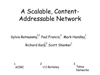
LAND : L ocality A ware N etworks for D istributed Hash Tables. Dahlia Malkhi The Hebrew University of Jerusalem Joint work with: Ittai Abraham and Oren Dobzinski . Motivation. Today ’ s Internet: Many lightweight clients (web browsers) Relatively simple servers (HTTP)

E N D
LAND:Locality Aware Networks for Distributed Hash Tables Dahlia Malkhi The Hebrew University of Jerusalem Joint work with: Ittai Abraham and Oren Dobzinski
Motivation • Today’s Internet: • Many lightweight clients (web browsers) • Relatively simple servers (HTTP) • Client-Server paradigm is suited for a world of thin clients which do not have a lot of bandwidth and computational power. • Tomorrow’s Internet ? • Most devices will have enough bandwidth and CPU to become both a client and a server (peer). • Users will have an active network presence.
Challenges • New Distributed Storage and Retrieval Services will face many challenges: • Scalability –number of users constantly increases. • Dynamism –unlike today’s web servers, peers will be constantly joining and leaving. • Congestion –Access to data is non-uniform and may cause hot spots. • Fault tolerance –availability and reliability of data. • Efficiency –systems should be resource efficient and provide the best performance (more on this later).
Overlay networks and distributed data structures • Hash tables: store and lookup by object id • Quorum systems: global search • Prefix lookup • SQL • Google • ?
Viceroy Overview • Viceroy, the first constant-degree distributed hash table [Malkhi, Naor, Ratacjzak, PODC 02] • LAND, the first peer-to-peer network and lookup algorithm that has worst case constant distortion [Abraham, Malkhi, Dobzinski SODA 2004] • A generic overlay network approach with implicit load balancing [Abraham, Awerbuch, Azar, Bartal, Malkhi, Pavlov, IPDPS 03] • A publish-subscribe mechanisms for scale-free graphs based on probabilistic quorums [Abraham, Malkhi, DISC 03] • Small-world DHTs on planar metrics [Abraham, Malkhi, 2003] • An optimal asynchronous resource discovery scheme [Abraham, Dolev, PODC 03] • Investigation of user privacy and anonymity [Bickson, Malkhi, 2003] • An efficient, localized scheme for estimating the number of nodes in a dynamic network [Horowitz, Malkhi, IPL 2003]
Overlay Networks for Finding Nearest Copy of Data • Nodes construct an overlay layer that allows to use new network architectures and services. • A Content Addressable Network allows to route to the target node by examining the object’s id. • If multiple copies of the same object exist then the closest copy should be accessed. • Complexity measures for Overlay Networks: • Number of hops from source node to target node. • Degree of the overlay network. • Amount of additional memory needed per object. • Adaptability: number of nodes that change their state each time a peer joins/leaves the system. • Load on nodes related to the locating task
Locality • Suppose a new DHT ensures each object will be found in 4 hops. • So a lookup could begin in Boston and go to Brazil, New Zealand, France and finally New York. • For some applications this is not a desired outcome.
Network models • The Internet • Fully connected weighted graph • Weight = ping latency (?) • Internet with geometric coordinates • Distance = geographic distance • Mobile network • Geometric space with limited transmission range • Arbitrary graphs
Distortion • Let c(s, t) be the distance from s to t • Let s=x1 x2…xk=tthe route from s to t • Distortion is the ratio betweenc(x1, x2) + … + c(xk-1, xk)andc(s, t)
2r The Model • Cost function c that forms a metric • c(x,y) ≥ 0 (positive), c(x,x)=0 (reflexive), c(x,y)=c(y,x) (symmetric) • Triangle inequality: c(x,y) + c(y,z) ≥ c(x,z) • Minimal distance between peers is 1. • N(x,r) denote the set of nodes at distance <r from x. • Growth Bounded Metric: • Actually, assume uniform density first r
LAND origins and related work • Based on the scheme of Plaxton, Rajaraman, Richa. “Accessing nearby copies of replicated objects in a distributed environment.”Theory of Computing Systems, 1999. • PRR ensures that the expected distortion is constant. • Tapestry and Pastry DHT’s are both based on the basic static PRR scheme. They enhance PRR by handling dynamic changes in the network. • More..
LAND architecture • A set of objects A. • Objects can be stored on any node. • Multiple nodes can keep a replica of each object. • Uniformly distributed hash function h(A). • Uniformly selected node identifiers • Nodes keep transient routing information about objects. Hashed-home here ? Resides here
Identifiers and links • Each node has n=log(N) identifier 2-bit digits • Node a1a2…an has n links • Link k `fixes’ k’th digit • Connects to closest node with identifier a1a2…ak-1[0-3]* • Link k property: • Found with probably 1/4k • Expected to be found within a ball with 4k nodes • Goes to distance 2k
Publish and lookup • Prefix-routing: fix one digit at a time • Publish object A at node t: • Leave reference “A;t” at each node en-route • Lookup A: route until reference to A found • Route distance: At most network diameter = 21 + 22 + … + 2n
Example of Publish: node t publishes Obj h(Obj)=101 t=*** w1=1** w2=10* w3=101 w3 t w1 w2
Problem 1: • Link distance could be more than expected • Solution: Emulate a shadow node • A shadow node that fixes digit k has links fixing digit k+1 • If a1a2..ak-1d* not found at distance 2k then look for a1a2..ak-1d[0-3]* and within 2(k+1)
Expected O(n) number of shadow nodes • Probability of emulating link k at most (1-1/4k) 4^k < e-1 • Bk+i– expected number of shadow nodes with prefix k+i • E[Bk+i] = E[Bk+i|Bk+i-1] = 2e-1E[Bk+i-1] = (2/e) i • Total expected number of shadow nodes starting with link k is constant
Problem 2: • Unbounded distortion; if target is very close, price is too high • Solution: `publish’ links • Step k in a publish route places reference in appropriate nodes in bigger neighborhood
Publish links • Denote 2k ≥ c(s,t) • k is the first such index • Step k of lookup route is at most 2(k+1) away (denote xk) • Step k of publish route is at most 2(k+1) away (denote wk) • c(xk , wk) ≤ 3*2(k+1) • Publish a k’th step to all nodes within distance 2(k+1)+2 with identifer matching k-prefix , so xk will contain a reference to wk
Example of Publish: node t publishes Obj h(Obj)=101 t=*** w1=1** w2=10* w3=101 For example: w1 publishes to nodes with id=1* within a distance proportional to distance(t, w1) w3 t w1 w2
Lookup Algorithm w3 t w1 w2 x4 x3 x2 x1 x0 x
Distortion • Route from s to xk • Plus distance from xk to wk • Plus route from wk to t • constant factor over distance from s to t • Distortion can be made close to 1 by increasing range of publish links
Summary of LAND properties • Guaranteed (small) constant distortion • Expected logarithmic node-degree • Simple analysis • Amenable to dynamic deployment
Dynamic maintenance • Find closest node to x: • From any node y, let Sn = {y} • Recursively, set Sk-1 = closest node among incoming prefix-(k-1) links into Sk • Closest is S1 • Correctness: • Let s be closest to x; route from s to y • Step k is within 2(k+1) distance • If Sk is closest to x with k-prefix match to Sn is within 2(k+1) distance, then so is Sk-1
Neighbor finding • From closest, route k steps, then back-track incoming links two steps, to find prefix-(k-2) links • Correctness: • Node k is 2(k+1) distance away • Incoming links are 2k+2 away, covering 2(k-2) away
2r Back to growth-bound model • N(x,r) denote the set of nodes at distance <r from x. • Growth Bounded Metric: r
Setting node Identifier and Level. • Set a radix B • Let M such that BM = N. • Id has M digits of radix B. • Denote A i (x) as the ball around x with α Bi nodes (e-αB<1) • A i (x) has constant numberof expected nodes with any specific length-i identifier.
Network links • Each node has M initial routers • Router in level k has links to routers in level k+1 : • router u with id a1,a2,…,ak,ak+1…aM and level k, maintains three types of links: • Neighbor– for each digit b in [0…B-1] a link to the closest node with id beginning with a1,a2,a3,…,ak,b and level k+1 inside the ball A k+1 (u). • Publish - a link to all nodes with id beginning with a1,a2,a3,…,akand level k+1 inside the ball A k+5 (u).
Example of Publish: Super-node t publishes Obj h(Obj)=abc t=*** w1=a** w2=ab* w3=abc For example: w1 publishes to routers with level 2 and id=ab* inside the ball A6(w1) w3 t w1 w2
Enforcing Locality withShadow Nodes • Recall: Neighbor– for each digit b in B a link to the closest node with id a1,a2,a3,…,ak,b and level k+1. • Want all neighbor links of a level k node u to be inside Ak+1(u). • For any b, if no b’th neighbor is in Ak+1(u) then u emulates a shsadow node v with id a1,a2,a3,…,ak,b and level k+1. • Node u establishes all of this shadow router’s network links. Including v’s neighbor links. • Recursively this process continues until all shadow nodes have all their links either close enough or emulated.
Variations and extensions • Two-tier architecture, constant expected node degree • Content Addressable Networks • Fault Tolerance
Two-hop stretch-3 DHT • Each node v has identifier h(v) • h() has sqrt(N) different values • Node v has links to: • log(N)*sqrt(N) closest nodes, so one of each value w.h.p • All nodes u with h(u)=h(v) • Routing from s to t in two hops: • Find node w with h(w)=h(t) • Find t • Stretch: • c(s, w) + c(w, t) ≤ c(s, t) + 2c(s, t)
Ai+1(y) Ai(y) Ai(x) Ai+1(x) Analysis:Balls • Recall Ai(x) is the smallest ball around x with α Bi M nodes (e-αB<1). • Suppose y in Ai(x) then: • Ai(y) in Ai+1(x) • Ai(x) in Ai+1(y) y x
Proof of Ai(y) in Ai+1(x) • Ai(y) is less than N(2ai(x),x) because it contains the ball Ai(x) • N(2ai(x),y) is less than N(4ai(x),x) by simple distances • N(4ai(x),x) is less than Ai+1(x) due to the growth restriction and the way we chose B • Proving Ai(x) in Ai+1(y) is very similar
ai+1(x) Ai(x) Ai+1(x) Growth of Balls • Recall Ai(x) is the smallest ball around x with α Bi nodes (e-αB<1). • Let ai(x) denote the radius of Ai(x) • ai+1(x) ≤ maxgrow ai(x) • ai+1(x) ≥ mingrow ai(x) ai(x)
Analysis:Distortion • The initial node is x looking for Obj. • x0=s is the closest super node. • w0=t is the closest super node holding Obj. • w0,w1,w2,.. is the sequence of nodes used to publish OBj. • x0,x1,x2,.. is the set of nodes fixing the bits to reach h(Obj), node xi has level i. • Xk is the first node that has a reference to OBj published by node wk-1. • Need to find bound on path x,x0,x1,x2,…,xk,wk-1,wk-2,…,w2,w1,w0=t compared to c(x,t).
Analysis:Distortion • For every i: • xi in Ai+1(s) and wi in Ai+1(t) • The path from s=x0 to xi is at most • Similarly for the path from t=w0 to wi • If t in Ak(s) then xk contains a reference to Obj • Distortion is
Analysis:Expected Degree • Expected number of virtual nodes emulated by a node is constant. • Expected number of publish links is constant. • Expected degree of regular nodes is constant. • Expected degree of super-nodes is logarithmic.
Expected number of emulated nodes is • The probability that a random node will be a neighbor link is 1/(Bl+1M). • The probability that a neighbor link will be found inside Al+1(u) is
Expected number of emulated nodes is • Let bl+i be the number of virtual nodes of level l+i. So bl=1. • E(bl+i | bl+i-1) = bl+i-1 B e-α. • Thus E(bl+i) = E(bl+i-1) B e-α. • By induction: E(bl+i) = (B e-α)i • Number of virtual nodes:
A Generic Scheme for Building Overlay Networks in Adversarial Scenarios Ittai Abraham (HUJI), Baruch Awerbuch (JHU), Yossi Azar (TAU), Yair Bartal (HUJI), Dahlia Malkhi (HUJI), Elan Pavlov (HUJI)
Dynamic Model • Suppose the set of node in the network is dynamically evolving. • Peers in the DHT are constantly leaving and joining the system. • Join: a new node wants to join the system, it initially has access to an existing node. • Leave: a node departures from the system, this departure can either be graceful (performing any necessary cleanup operation) or sudden. • Low degree overlay network helps reduce overhead in the event of join/leave. • This process may cause network imbalance.
Coping with Imbalance • Solution 1 [FS 01, FSGKS 02]: Assume population is always in between n and ½n (censorship). • Solution 2 [Chord 01, CAN 01]: Execute periodic global overhaul operations for rebalancing. • Problem: global operations are costly and may totally shut down the service. Impractical for large systems. • Solution 3 [Pastry 01, Tapestry 01]: Assume population change is a random process that maintains the initial randomness. • Problems: • DHT systems may have hot spots, and many nodes entering may use the same access node. • Failures tend to be correlated. • A malicious adversary may try to disrupt the network by causing imbalance.
Load Balancing Against an Adversary • In this work we allow an adversary to adaptively choose: • The order of join and leave events. • For leave events: which node to remove. • For join events: what is the access node of the newly added node. • Against such an adversary we employ load balancing upon arrival and departure. • After each event the overlay network executes protocols for rebalancing the network.
Problem Statement • Devise an overlay network and join leave protocols, with the following properties: • Efficient decentralized routing. • Low cost for rebalancing join and leave events against an adversary.
Generic Solution for Child-Neighbor Commutative Families • Consider a set of graphs G1, G2, G3, … • With mapping pi from Gi+1 on to Gi. • Denote child function ci(u)={v| pi(v)=u} • Denote neighbor function n(u)={v|(u,v)E} • Child-Neighbor commutative property: For every u: n(c(u))=c(n(u))
The Hypercube as an example • The hypercube Gi :has 2^i nodes each node’s id is a binary string of length i. • A node in Gi :has links to the i nodes that have only one bit different in their id. • The child function is c(x)={x0,x1} • Example of Child-Neighbor commutative property for node 10 in G2. • n(10)={11,00}, c(n(10))={111,110,001,000} • c(10)={100,101}, n(c(10))={000,110,101,001,110,100}
The Dynamic Graph • For this talk we focus on the Dynamic Hypercube (in paper de Bruijn, Butterfly). • Start with two nodes with id 1, 0. • Split: change node with id x into nodes x0, x1. • Merge: change two twin nodes x0, x1 into node with id x. • Not all of the nodes n(x) exist in the network. • Edges: A node x connects to all the nodes whose id is a prefix of n(x) or n(x) is a prefix of their id. • For example: Node 110 would link to all nodes in the dynamic graph whose id is a prefix of {010, 100, 111} for instance: 01, 100101, 1000, and 111.