Download
1 / 71
740 likes | 990 Views
Switching and Forwarding. 3.1 Switching and Forwarding 3.2 Bridges and LAN Switches 3.3 Cell Switching (ATM) 3.4 Implementation and Performance. Two limitations on the directly connected networks limit on how many hosts can be attached, examples

E N D
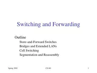
Switching and Forwarding 3.1 Switching and Forwarding 3.2 Bridges and LAN Switches 3.3 Cell Switching (ATM) 3.4 Implementation and Performance
Two limitations on the directly connected networks • limit on how many hosts can be attached, examples • only two hosts can be attached to a point-to-point link • the Ethernet specification allows no more than 1,024 hosts
limit on how large of a geographic area a single network can serve, examples • an Ethernet can span only 2,500 m • wireless networks are limited by the ranges of their radios • point-to-point links can be quite long
Goal • build networks that can be global in scale • Problem • how to enable communication between hosts that are not directly connected • Solution • computer networks use packet switches to enable packets to travel from one host to another, even when no direct connection exists between those hosts
Packet switch • a device with several inputs and outputs leading to and from the hosts that the switch interconnects • Core job of a switch • take packets that arrive on an input and forward (or switch) them to the right output so that they will reach their appropriate destination
A key problem that a switch must deal with is the finite bandwidth of its outputs • if packets destined for a certain output arrive at a switch and their arrival rate exceeds the capacity of that output, then we have a problem of contention • the switch queues (buffers) packets until the contention subsides, but if it lasts too long, the switch will run out of buffer space and be forced to discard packets • when packets are discarded too frequently, the switch is said to be congested
3.1 Switching and Forwarding • Switch • a multi-input, multi-output device, which transfers packets from an input to one or more outputs • star topology • switched networks are more scalable (i.e., growing to large numbers of nodes) than shared-media networks because of the ability to support many hosts at full speed
Scalable Networks • The figure shows the protocol graph that would run on a switch that is connected to two T3 links and one STS-1 SONET link Example protocol graph running on a switch
A switch forwards packets from input port to output port • Port selected based on address in packet header • Advantages • cover large geographic area (tolerate latency) • support large numbers of hosts (scalable bandwidth)
How does the switch decide on which output port to place each packets? • general answer • it looks at the header of the packet for an identifier that it uses to make the decision • three common approaches • datagram (or connectionless) approach • virtual circuit (or connection-oriented approach) • source routing
3.1.1 Datagram Switching • Sometimes called connectionless model • Analogy: postal system • No connection setup phase • no round trip delay waiting for connection setup • a host can send data as soon as it is ready
Each packet is forwarded independently of previous packets that might have been sent to the same destination • two successive packets from host A to host B may follow completely different paths (perhaps because of a change in the forwarding table at some switch in the network)
A switch or link failure might not have any serious effect on communication if it is possible to find an alternate route around the failure and to update the forwarding table accordingly • Since every packet must carry the full address of the destination, the overhead per packet is higher than for the connection-oriented model
Source host has no way of knowing if the network is capable of delivering a packet or if the destination host is even up and running • Each switch maintains a forwarding (routing) table
Example • the hosts have addresses A, B, C, and so on • a switch consults a forwarding table (routing table) to decide how to forward a packet
The table shows the forwarding information that switch 2 needs to forward datagrams
3.1.2 Virtual Circuit Switching • Sometimes called connection-oriented model • Analogy: phone call • Explicit connection setup (and tear-down) phase • it requires that a virtual connection from the source host to the destination host is set up before any data is sent • Typically wait full RTT (Round Trip Time) for connection setup before sending first data packet
If a switch or a link in a connection fails • the connection is broken and a new one needs to be established • Subsequence packets follow same circuit • Each switch maintains a Virtual Circuit (VC) table
Entry in the VC table on a single switch contains • a virtual circuit identifier (VCI) • uniquely identifies the connection at this switch • which will be carried inside the header of the packets that belong to this connection
an incoming interface • on which packets for this VC arrive at the switch • an outgoing interface • in which packets for this VC leave the switch • a potentially different VCI that will be used for outgoing packets
Two classes of approaches to establish connection state • Permanent Virtual Circuit (PVC) • Switched Virtual Circuit (SVC)
Permanent Virtual Circuit (PVC) • administrator configures the state, in which case the virtual circuit is “permanent” • administrator can also delete the state, so a permanent virtual circuit (PVC) might be thought of as a long-lived, or administratively configured VC
Switched Virtual Circuit (SVC) • a host may set up and delete a VC by sending messages without the involvement of a network administrator • this is referred to as signaling, and the resulting virtual circuits are said to be switched • an SVC should more accurately be called a “signaled” VC, since it uses signaling (not switching) to distinguish an SVC from a PVC
Example • assume that a network administrator wants to manually create a new virtual connection from host A to host B • two-stage process • connection setup • data transfer
(11) (7) (5) (4) An example of a virtual circuit network
The administrator picks a VCI value that is currently unused on each link for the connection • suppose • VCI = 5, the link from host A to switch 1 • VCI = 11, the link from switch 1 to switch 2 • VCI = 7, the link from switch 2 to switch 3 • VCI = 4, the link from switch 3 to host B
VC table entry at switch 1 VC table entry at switch 2 VC table entry at switch 3
Hop-by-hop flow control • each node is ensured of having the buffers it needs to queue the packets that arrive on that circuit • example, an X.25 network-a packet-switched network that uses the connection-oriented model
X.25 network employs the following three-part strategy • buffers are allocated to each virtual circuit when the circuit is initialized • the sliding window protocol is run between each pair of nodes along the virtual circuit, and this protocol is augmented with flow control to keep the sending node from overrunning the buffers allocated at the receiving node
the circuit is rejected by a given node if not enough buffers are available at that node when the connection request message is processed
Examples of virtual circuit technologies • Asynchronous Transfer Mode (ATM) • Frame Relay, e.g., Virtual Private Network (VPN) • Frame Relay operates only at the physical and data link layers
3.1.3 Source Routing • Neither virtual circuits nor conventional datagrams • All the information about network topology that is required to switch a packet across the network is provided by the source host
Various ways to implement source routing • method1 • put an ordered list of switch ports in the header and to rotate the list so that the next switch in the path is always at the front of the list • for each packet that arrives on an input, the switch would read the port number in the header and transmit the packet on that output
Source routing in a switched network (where the switch reads the rightmost number)
method2 • example, rather than rotate the header, each switch just strip the first element as it uses it • method3 • have the header carry a pointer to the current “next port” entry, so that each switch just updates the pointer rather than rotating the header
Three ways to handle headers for source routing: (a) rotation, (b) stripping, and (c) pointer. The labels are read right to left
3.2 Bridges and LAN Switches • LANs have physical limitations (e.g., 2500m) • Bridge (LAN switch) • connect two or more LANs • Extended LAN • a collection of LANs connected by one or more bridges • accept and forward strategy (accept all frames transmitted on either of the Ethernets, so it could forward them to the other)
3.2.1 Learning Bridges • Do not forward when unnecessary • whenever a frame from host A that is addressed to host B arrives on port 1, there is no need for the bridge to forward the frame out over port 2
How does a bridge come to learn on which port the various hosts reside? • each bridge inspects the source address in all the frames it receives • when host A sends a frame to a host on either side of the bridge, the bridge receives this frame and records the fact that a frame from host A was just received on port 1 • in this way, the bridge can build a table just like the following table
3.2.2 Spanning Tree Algorithm • Problem: extended LAN has a loop in it • frames potentially loop through the extended LAN forever • example • bridges B1, B4, and B6 form a loop
Solution: bridges run a distributed spanning tree algorithm • spanning tree is a subgraph of a graph that covers (spans) all the vertices, but contains no cycles
Example of (a) a cyclic graph; (b) a corresponding spanning tree