Download
1 / 41
410 likes | 594 Views
Exponential random graph ( p *) models for social networks Workshop Harvard University February 2002 Philippa Pattison Garry Robins Department of Psychology University of Melbourne Australia Plan for the workshop Model construction: dependence graphs

E N D
Exponential random graph (p*) models for social networks • Workshop • Harvard University • February 2002 • Philippa Pattison • Garry Robins • Department of Psychology • University of Melbourne • Australia
Plan for the workshop • Model construction: dependence graphs • Dyadic independence and Bernoulli graph models • Example: The network structure of a US law firm • Markov random graphs • Example: Mutual work ties among the lawyers • Estimation • Pseudo-likelihood estimation • Monte Carlo maximum likelihood • Incorporating individual level variables • Directed dependence graphs • Social selection models • Example: Advice ties among the lawyers • Further steps
General framework for model construction • 1. Regard each network tie as a random variable (often binary) Xij = 1 if there is a network tie from person i to person j = 0 if there is no tie for i, j members of some set of actors N. A directed network: Xij and Xji are distinct. A non-directed network: Xij = Xji X … matrix of all variables x … matrix of observed ties (the network)
General framework for model construction • 2. Formulate a hypothesis about interdependencies and construct a dependence graph • 3. The Hammersley-Clifford theorem produces a general model : • each parameter corresponds to a configuration in the network • 4. Consider homogeneity constraints: should some parameters be equal? • 5. Estimate model parameters
Dependence graphs • Spatial statistics (Besag, 1974) • Spread of a contagious disease in a field of plants. • Whether or not a plant has the disease in part depends on whether nearby plants have the disease. • The probability of a plant having the disease is conditionally dependent on whether neighbouring plants have the disease. • What counts as neighbouring plants?
10 11 12 1 2 3 4 6 5 9 7 8 How to represent neighbours? • For example: a 2-dimensional lattice
Z10 Z11 Z12 Z1 Z2 Z3 Z4 Z6 Z5 Z9 Z7 Z8 More abstractly … a dependence graph! • Random variables • Zi = 1 if plant i has the disease • Zi = 0 if plant i does not have the disease
And then ... • Besag (1974) used the Hammersley-Clifford theorem to derive a probabilistic description of the entire system • in terms of the hypothesised local dependencies. • Cliques of the dependence graph. • The sufficient statistics of the model are all the combinations of variables that are all neighbours of each other.
Z10 Z11 Z12 Z1 Z2 Z3 Z4 Z6 Z5 Z9 Z7 Z8 Cliques of the dependence graph • Z7, Z8, Z12 are all neighbours of each other. • Whether plant 7 has the disease depends not only on whether plant 8 or plant 12 has the disease, but also on whether both 8 and 12 have the disease simultaneously.
For social networks • The dependence graph represents the contingencies among network variables Xij. • The cliques of the dependence graph represent local configurations in the network. (a configuration is a small subgraph of the network) • There is one parameter in the model for each clique. (ie one parameter for each configuration.) • The model then is an expression of the probability of the network expressed in terms of local configurations.
i j i j i j Example: Dyadic independence models • Hypothesis about a possible local process: • Whether person i considers person j a friend is contingent on whether person j considers person i a friend.
The Hammersley-Clifford theorem • Pr(X= x) = p*(x) = (1/c) exp{Sall cliquesAzA} • where: the summation is over all cliques A; zA = PxijÎAxij is the network statistic corresponding to the clique A; A is the parameter corresponding to clique A; c = SX exp{SAAzA(x)} is a normalising constant • (Besag, 1974)
For dyadic independence • Cliques: {Xij}, {Xji}, {Xij, Xij} • So: Pr(X= x) = (1/c) exp{Sall cliquesAzA} • with zA = PAxij • becomes: • Pr(X= x) = (1/c) exp{Si,jij xij +Si,jij,ji xijxji } • Homogeneity: ij= ; ij,ji = • Pr(X= x) = (1/c) exp{Si,jxij +Si,jxijxji } • = (1/c) exp{L+ M} • where L is no. of ties, M is no. of mutual ties
Homogeneity • The model cannot be estimated (unidentifiable) unless some parameters are equated: • ie, assume that certain effects are the same for all (or at least large parts) of the network • eg, a single tendency for mutuality across the entire network. • Homogeneity of isomorphic network configurations • parameters equated for the same types of configuration ignoring the numbering on the nodes • statistics become the counts of the configurations in the network • parameter interpretation: tendency for the configuration to be present in the network, given the other configurations. • Isomorphic configurations within blocks
i j Xij Xkl Bernoulli graphs: the simplest dependence structure • Dependence assumption: all ties are independent. • Dependence graph:
Bernoulli block models • Suppose actors are either in block 1 or 2 • Hammersley-Clifford: Pr(X= x) = (1/c) exp{Si,jij xij } • Block homogeneity: ij = 11 if i and j both in block 1 ij = 12 if i in block 1 and j in block 2, etc. • Pr(X= x) = (1/c) exp{11 L11+12 L12+21 L21+22 L22} where Lrs is the number of edges from block r to block s.
Example: The network structure of a US law firm(Lazega & Pattison, 1999) • Respondents: All 71 lawyers Blocks: 36 partners (block 1), 35 associates (block 2) • CoworkerandAdvice ties: • The general question: • How is collective participation organised? • Small, flexible, and temporary work-teams must be able to form quickly and cooperate efficiently in order to react to complex and non-standard problems. • Regularities in local patterns of exchange provide one possible solution.
Bernoulli and dyad-independent models for advice ties • a. Homogeneous Bernoulli: Pr(X= x) = (1/c) exp (L) • b. Bernoulli blockmodel: • Pr(X= x) = (1/c) exp{11 L11+12 L12+21 L21+22 L22} • c. Homogeneous Dyad-independent: • Pr(X= x) = (1/c) exp{L+ M} • d. Dyad-independent block • Pr(X= x) = (1/c) exp{Sr,s=1,2rs Lrs+ M} • e. Dyad-independent block with block reciprocity parameters: • Pr(X= x) = (1/c) exp{Sr,s=1,2(rs Lrs+rsMrs)}
Results:Using pseudolikelihood estimation (to come)PL deviance is a measure of fitMAR = Mean absolute residual • PL deviance MAR Parameters • a. Bernoulli model 4677.8 .294 1 • b. Bernoulli block 4341.1 .276 5 • c. Homogeneous dyad-independent model 4391.1 .275 2 • d. Dyad-independent block model 4072.6 .258 5 • e. Dyad-indpt block with block reciprocity • 4071.2 .257 8
Parameter estimates for model c • Advice ties: (P=Partner, A=Associate) • Parameter MPLE • 11 -1.34 Density of ties in P • 12 -3.51 Ties from P to A • 21 -1.53 Ties from A to P • 22 -1.98 Density of ties in A • 1.52 Reciprocity
Markov Random Graphs • Dyadic independence is an unrealistic assumption • Both theoretically and empirically. • Markov Dependencies (Frank & Strauss, 1986) • Assume that a tie from i to j is contingent only on other ties involving person i and person j. • network ties assumed conditionally dependent if and only if they share a common actor • There is an edge (Xij, Xkl) in the dependence graph if and only if {i,j} {k,l}
Xjk Xij Xkj Xji Xki Xik Markov dependence graph for a directed network • Cliques of size 1 or 2 : • { Xij } • { Xij ,Xji } • { Xij ,Xik } • { Xij ,Xjk } • { Xij ,Xkj }
Xjk Xij Xkj Xji Xki Xik Markov dependence graph for a directed network • Cliques of size 3 : • 1. Stars • { Xij , Xik , Xil } • etc • 2. Triads • Transitive triads • { Xij ,Xjk , Xik } • 3-Cycles • { Xij ,Xjk , Xki } • etc
Parameters for a homogeneous Markov random directed graph model NB: Bernoulli models- Density only; Dyad independent - Density plus reciprocity
Interpretation of Markov random graph models • Broadly, positive parameter indicates a high occurrence of the associated configuration. • But the effects are marginal to each other. • A positive parameter indicates a greater number of the configuration than expected, given the observation of other configurations • Interpret a higher order parameter in relation to its lower order constituents. • e.g. interpret cyclic triads in relation to 2-mixed-stars (2-paths): Positive cyclic parameter suggests presence of more cycles than expected from the number of 2-paths.
Example: Markov random graph model for mutual work ties among the lawyers • Model parameters -2LPL MAR • _________________________________________ • 1. Edge (density) 2119.0 .258 • 2. edge, 2-star, 3-star, triangle 1760.8 .213 • _________________________________________ Lazega AdviceWork.ppt
Pseudo-likelihood estimation:an approximate technique • Conditional form of the Hammersley-Clifford theorem: • where: • (1) The sum is over all cliques A that contain Xij; • (2) A is the parameter corresponding to clique A; • (3) dA(ij) is the change statistic • the change in the value of the network statistic zA(x) when xij changes from 1 to 0 • Note: this version of the theorem takes the form of a conditional logistic regression.
Calculating the change statistic • Eg: Markov random graph model for a nondirected network. • Graph statistics: edges, 2-stars, 3-stars, triangles. • Set up standard logistic regression file: • “Cases” are each possible tie (i, j). • Variables: Xij , edges, 2-stars, 3-stars, triangles. • Eg, to calculate 2-stars value for each (i, j): • count 2-stars in the network when Xij =1 • count 2-stars in the network when Xij =0 • take the difference. • Predict Xij =1in a standard logistic regression from the other variables
Some warnings • This looks like a logistic regression: It is not!! • The standard errors are at best approximate (probably too small). • Do not rely on the Wald statistic. • You cannot assume the pseudo-likelihood deviance is asymptotically chi-squared • But the PL deviance still indicates how well the model fits the observed network. • If a variable does not contribute “substantially” to the PL deviance, maybe exclude it? • But maybe keep lower order variables in the model if higher order variables are important. • Report PL deviance and mean absolute residual.
Monte Carlo Maximum Likelihood Estimation • Some recent developments in this area, eg Snijders 2002 • Degenerate regions in the parameter space • So far, studies only involve simple non-directed Markov random graph models • Possible importance of model specification • Implications for Pseudolikelihood estimation • Do not treat PL as hypothesis testing; it is more exploratory. • More work is needed to determine types of models, and regions of parameter space, for which we can be confident about PL estimation. • Nevertheless, PL is convenient, and for complex models is still our only available estimation technique
Incorporating individual level variables • Attribute variables:e.g. sex, rank, attitudes • Yi = 1 if actor i possesses the attribute (e.g. actor i is female) • Yi = 0 otherwise • Example: Social selection models (Robins, Elliott & Pattison, 2001). • Similarity or homophily hypothesis: There is a propensity for a tie to develop between actors with similar attributes.
Attribute variables Network variables (possibly some non-directed dependencies among network variables) Directed dependence graphs • One type of variable predictive of another • Two block chain graphs Example: Dyadic independence Markov attribute models Yi Yj Xij Xji
Yi Xki Yj Xik Xij Xji Xkj Xjk Markov graph - Markov attribute models
i j k Markov graph - partial dependent attribute models • A possible tie between two people is contingent on a third person’s attribute if the third person is tied to at least one of the first two. E.g. k’s attribute possibly shapes whether there is a tie from i to j
Configurations and estimates for reduced partial dependence model
Other applications of directed dependencies • Social influence models • Robins, Pattison & Elliott (2001) • Discrete time models • Robins & Pattison (2001) • Tripartite graphs • Mische & Robins (2002)
Further stepsPattison & Robins (2002) • Partial dependence models: • observed ties create new neighbourhoods • longer range dependencies • longer cycles (eg generalized exchange)
Xjk Xij Xkj Xji Xki Xik Further stepsPattison & Robins (2002) • Setting structures: • A setting: a subset of possible ties • potential "site of social action" • e.g., focus, Feld (1981) • network-domain (White, 1995) • Limits the scope of the dependencies in the dependence graph: