Download

1 / 16
170 likes | 193 Views
Instrumental Variables. Methods of Economic Investigation Lecture 15. Last Time. Introduction to Instrumental Variables Correlation with variable of interest Exclusion restriction Interpretation of IV with homogeneous treatment effects Gives us a Wald estimate

E N D
Instrumental Variables Methods of Economic Investigation Lecture 15
Last Time • Introduction to Instrumental Variables • Correlation with variable of interest • Exclusion restriction • Interpretation of IV with homogeneous treatment effects • Gives us a Wald estimate • Nice/well-defined properties of OLS
Today’s Class • Uses for 2SLS • Experiments with compliance issues • Omitted Variable Bias • Heterogeneous Treatment Effects • LATE framework • Interpretation
Review of Instrumental Variables • Two characteristics • Instrument (Z) is correlated with (S) • Must be that S is alwaysincreasing (or always decreasing) • If it changed signs, then the first stage prediction wouldn’t work • Instrument (Z) is uncorrelated with other determinants of the outcome (Y) • This means Z is uncorrelated with unobservables that affect Y • The only way Z affects Y is through S
Steps to Estimate IV-1 • Step 1: The Structural Equation Y =ρS + η • Problems: S correlated with η • OLS estimates won’t recover causal effect of S on Y • Step 2: Find an Instrument • Correlated with S • Uncorrelated with η (and so uncorrelated with the unobservables)
Steps to Estimate IV-2 • Step 3: Estimate the First Stage S = πZ + ν • Can estimate this with OLS • Want to test to see if π is significant—will return to this in the case of weak instruments where α is close to zero • Step 4: Obtain the fitted values • This is the component of S that is unrelated to the error term in the structural equation
Steps to Estimate IV -3 • Step 5: Estimate the Second Stage • This is using the fitted value, i.e. the predicted value of S given the instrument Z • The fitted value captures the component of S that is uncorrelated with the error • If we want to recover β take the OLS estimate from the second stage b and divide it by the coefficient from the first stage α
Various uses for IV Goal: Average Effect of S on Y (ATE) Omitted Variable Non-Experimental Experimental Perfect Compliance Imperfect Compliance Matching Diff-in-diff IV Fixed Effects IV Perfect Compliance Imperfect Compliance Measurement Error IV IV
Things to worry about • Is my instrument really uncorrelated with other determinants of the outcome? • How do I interpret my IV estimate? What if I think there are heterogeneous treatment effects? • How strong does my first stage have to be for this to all work? We’ll deal with each of these issues
Can we test the exclusion restriction • This is the assumption of the model and often cannot be formally tested • The reduced form gives some information on the reasonableness of the assumption • Knowing π and the OLS biased estimated of ρ we might gut check how reasonable it is for the only effect of Z to be through S • If we have multiple instruments, we can test using the overidentification test
Overidentification • Model is overidentified if we have: • # instruments variables > # endogenous variables • Models with exactly same number of instruments as endogenous variables are just identified • If the model is overidentified we can test the quality of the fit
Testing Model Fit • Suppose we have Q instruments and define (this is our first stage RHS variable) • Define and as before • The residuals from the second stage can be defined as:
2SLS Residual Terms • We assume that η is orthogonal to Z so that E[Ziη(Γ)]=0 • The sample analog of this is • In finite samples, this won’t be exactly zero • 2SLS fits the value of Γ making this closest to zero • This has an asymptotic distribution of where
The Minimand • There is an underlying Method of Moments way to illustrate this but we’ll ignore that for now. • Basic idea is to minimize the quadratic form of the vector mN(Γ) • The optimal weighting matrix to estimate this is Λ-1 and then the equation to be minimized is:
The Overidentification Test • Intuition: is mn(g) close enough to zero for us to believe that Z uncorrelated with the error (other unobservable stuff) • Null hypothesis: E[ηZ]=0 distributed Χ2(Q-1) • Can also test this directly • Estimate the just-identified version for the Q instruments • Test that the estimate coefficients are statistically indistinguishable
Next time • Issues with IV • Heterogeneity • Weak Instruments