Instrumental Variables

1. Instrumental Variables Based on Greene’s Note 13

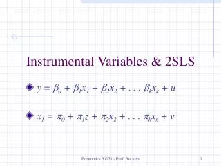
2. Instrumental Variables • Framework: y = X + , K variables in X. • There exists a set of K variables, Z such that plim(Z’X/n) 0 but plim(Z’/n) = 0 The variables in Z are called instrumental variables. • An alternative (to least squares) estimator of  is bIV = (Z’X)-1Z’y • We consider the following: • Why use this estimator? • What are its properties compared to least squares? • We will also examine an important application

3. IV Estimators Consistent bIV = (Z’X)-1Z’y = (Z’X/n)-1 (Z’X/n)β+ (Z’X/n)-1Z’ε/n = β+ (Z’X/n)-1Z’ε/n  β Asymptotically normal (same approach to proof as for OLS) Inefficient – to be shown.

4. LS as an IV Estimator The least squares estimator is (X X)-1Xy = (X X)-1ixiyi =  + (X X)-1ixiεi If plim(X’X/n) = Q nonzero plim(X’ε/n) = 0 Under the usual assumptions LS is an IV estimator X is its own instrument.

5. IV Estimation Why use an IV estimator? Suppose that X and  are not uncorrelated. Then least squares is neither unbiased nor consistent. Recall the proof of consistency of least squares: b =  + (X’X/n)-1(X’/n). Plim b =  requires plim(X’/n) = 0. If this does not hold, the estimator is inconsistent.

6. A Popular Misconception A popular misconception. If only one variable in X is correlated with , the other coefficients are consistently estimated. False. The problem is “smeared” over the other coefficients.

7. The General Result By construction, the IV estimator is consistent. So, we have an estimator that is consistent when least squares is not.

8. Asymptotic Covariance Matrix of bIV

9. Asymptotic Efficiency Asymptotic efficiency of the IV estimator. The variance is larger than that of LS. (A large sample type of Gauss-Markov result is at work.) (1) It’s a moot point. LS is inconsistent. (2) Mean squared error is uncertain: MSE[estimator|β]=Variance + square of bias. IV may be better or worse. Depends on the data

10. Two Stage Least Squares How to use an “excess” of instrumental variables (1) X is K variables. Some (at least one) of the K variables in X are correlated with ε. (2) Z is M > K variables. Some of the variables in Z are also in X, some are not. None of the variables in Z are correlated with ε. (3) Which K variables to use to compute Z’X and Z’y?

11. Choosing the Instruments • Choose K randomly? • Choose the included Xs and the remainder randomly? • Use all of them? How? • A theorem: (Brundy and Jorgenson, ca. 1972) There is a most efficient way to construct the IV estimator from this subset: • (1) For each column (variable) in X, compute the predictions of that variable using all the columns of Z. • (2) Linearly regress y on these K predictions. • This is two stage least squares

12. Algebraic Equivalence • Two stage least squares is equivalent to • (1) each variable in X that is also in Z is replaced by itself. • (2) Variables in X that are not in Z are replaced by predictions of that X with all the variables in Z that are not in X.

13. 2SLS Algebra

14. Asymptotic Covariance Matrix for 2SLS

15. 2SLS Has Larger Variance than LS

16. Estimating σ2

17. Measurement Error y = x* +  all of the usual assumptions x = x* + u the true x* is not observed (education vs. years of school) What happens when y is regressed on x? Least squares attenutation:

18. Why Is Least Squares Attenuated? y = x* +  x = x* + u y = x + ( - u) y = x + v, cov(x,v) = -  var(u) Some of the variation in x is not associated with variation in y. The effect of variation in x on y is dampened by the measurement error.

19. Measurement Error in Multiple Regression

20. Twins Application from the literature: Ashenfelter/Kreuger: A wage equation that includes “schooling.”

21. Orthodoxy • A proxy is not an instrumental variable • Instrument is a noun, not a verb