Download
1 / 44
440 likes | 655 Views
Instrumental Variables (IV). Introduction to IV methods Successful application of IV: estimating treatment effects Interpretation of IV: What does IV estimate? Problems with IV: Weak instruments and reporting error. 1. Introduction to IV methods.

E N D
Instrumental Variables (IV) • Introduction to IV methods • Successful application of IV: estimating treatment effects • Interpretation of IV: What does IV estimate? • Problems with IV: Weak instruments and reporting error
1. Introduction to IV methods Problem: Estimate effect of treatment (T) on outcome (Y). i.e., estimate 1 in: (1) Yi = 0 + Ti1 + i == Xi + i (X=[1 T]) For simplicity, suppose: • Dichotomous treatment variable: T=1 if treated, 0 otherwise • Homogeneous treatment effect (1) • Linear • No covariates
OLS Estimates of Treatment Effect Least-squares estimate of equation (1) yields standard "experimental" estimator: e.g. difference in means between treatment and control. Key assumption of OLS is X (the treatment) is uncorrelated with ε (the unobserved determinants of the outcome):
Problem With OLS Estimates Key OLS assumption unlikely to hold because treatment related to omitted factors (W) influencing outcome. i.e. suppose we partition such that = W + , where E(X')=0. Then the validity of OLS estimates of 1 require treatment to be uncorrelated with omitted variables: E(T')=0 ==> E(T'W) = 0 ==> E(W|T=1) = E(W|T=0) ==> distribution of W must be “balanced”
Four Solutions to this Problem 1) Randomized Controlled TrialRCT is designed to ensure key OLS assumption: E(T')=E(T'W)=0. 2) “Natural” Experiments Attempt to mimic RCTs: Find similar observations with different treatment for “arbitrary” reasons (e.g. regulatory rules, law changes).♦ “Difference-in-Difference” estimates♦ Discontinuity design
Four Solutions to this Problem (cont.) • Adjustment for Observable Differences Attempt to condition on sufficient W's s.t. E(T')=0 treatment is random/ignorable conditional on W Then estimate directly by least squares: (1’) Y = 0 + T1 + W + Variants on this approach include: ♦ Matching, Case-Control ♦ Regression ♦ Fixed effects (sibling/person as own control) ♦ Propensity score
Four Solutions to this Problem (cont.) • Instrumental Variables (IV) Suppose exists instrumental variable (Z) that is: (A1) correlated with treatment: E(Z'T) 0 (A2) Uncorrelated with residual: E(Z')=0 Basis for IV estimator: Variants on this approach include: ♦ 2 Stage Least Squares (2SLS) ♦ Limited Information Maximum Likelihood (LIML) ♦ General Method of Moments (GMM) ♦ Sample selection corrections (“Heckit”)
A Simple IV Example If Z is dichotomous (0,1) and no covariates, simple interpretation: = (Difference in mean outcomes)/(difference in treatment rate) ♦ Wald estimator ♦ Analagous to randomization ♦ Key assumption: E(W|Z=1) = E(W|Z=0) ♦ If small treatment difference, estimate can be fragile: “balance on the head of a pin!”
2. Successful application of IV:estimating treatment effects in AMI McClellan, M., B. McNeil and J. Newhouse, JAMA, 1994. "Does More Intensive Treatment of Acute Myocardial Infarction Reduce Mortality?” ♦ Medicare claims data, elderly with heart attack (AMI), 1987-91 ♦ Treatment: Cardiac Catheterization (marker for aggressive care) ♦ Outcome: Survival to 1 day, 30 days, 90 days, etc. ♦ Instrument: Is nearest hospital a catheterization hospital? Differential Distance = (distance to nearest cath) - (distance to nearest non-cath) based on zipcode of residence, zip code of hospital
Is Differential Distance a Good Instrument? • Correlated with treatment (Cath)? Yes. ♦ 26.2% get Cath if nearest hospital is Cath hospital ♦ 19.5% get Cath if nearest hospital is not Cath hospital 2. Uncorrelated with unobserved patient severity? Never sure!But unrelated to observable patient severity in claims:
Major Findings of McClellan et al. • Least squares dramatically overstates treatment effect, because Cath associated with fewer risk factors. ♦ 1-year mortality is 30% lower (17% vs. 47%) if Cath ♦ OLS estimate is 24%, adjusting for observable risk factors 2. IV estimates suggest Cath associated with 5-10 percentage point reduction in mortality; nearly all in 1st day.
Validating McClellan et al. Recent work replicates & validates earlier work using: 1. more comprehensive control variables 2. alternative instruments: McClellan and Noguchi, 1998 (Tables 1 & 2 below) Geppert, McClellan and Staiger, 2001 (Table 4 below) -- Data from Cooperative Cardiovascular Project (CCP) Chart data for appx. 180,000 AMI patients from 1994-95 Linked Medicare claims data -- Treatments and outcomes of AMI in elderly as in earlier work -- Instruments: (1) Differential distance (2) Variation in hospital Cath rate (>4000 dummies)
Key Validation Questions • Are severity measures unobserved in claims data uncorrelated with instrument (differential distance)? • Are OLS results closer to IV with more extensive controls? • Are IV results robust to more extensive controls? • Are IV results robust to alternative instruments?
Conclusions of Validation • Measured individual covariates can be used to assess bias of alternative methods for estimating treatment effects with observational data. • Methods that attempt to adjust for observable differences are quite sensitive to the use of more detailed chart data, and yield biased estimates of treatment effects in commonly available datasets. • IV methods for evaluating AMI treatment are not sensitive to the use of more detailed chart data, and appear to have minimal bias.
Growing number of applications of IV using a variety of instruments n Geography as an instrument (distance, rivers, small area variation) n Legal/political institutions as an instrument (laws, election dynamics) n Administrative rules as an instrument (wage/staffing rules, reimbursement rules, eligibility rules) n Naturally occurring randomization (draft, birth timing, lottery, roommate assignment, weather)
3. Interpretation of IV:What does IV estimate? • What if the treatment effect is heterogeneous? - e.g. depends on patient severity- Then what does IV estimate? Effect for what population?- Angrist, Imbens and Ruben (1996) give careful answer. • Think of RCT’s - Criterion for inclusion in trial - Estimate treatment effect in well-defined population - Always issues of external validity (to general population) • Analogous issues arise with IV estimates - Who are the “marginal” patients (or “compliers”), whose treatment is effected by the instrument? - IV estimates treatment effect for these “marginal” patients. - Often not estimating treatment effect in general population.
Who Is the Marginal Patient? Example: McClellan, McNeil, Newhouse (1994) Who are being treated? Conceptually, the shaded areas below.
Who Is the Marginal Patient? So we would expect: 1. Patients with most to gain are always treated. 2. “Marginal” patients tend to have smaller effects of the treatment. 3. IV like RCT on patients thought to be least appropriate for treatment. 4. Average treatment effect among all those being treated may be higher.
Identifying “Compliers” Key issue in interpreting IV is identifying the “compliers”, i.e. the margin on which your instrument is working. In practice, three types of evidence are used for this purpose: • What range of variation in treatment variable is generated?- Does instrument identify groups with wide or narrow range of treatment?- For continuous treatment (e.g. dose), does instrument have effects throughout distribution or in narrow range? • Does instrument have larger effect on odds-ratio of treatment among some sub-populations in the sample?
Identifying “Compliers” (cont.) • When instrument increases treatment rate, does it also affect the average characteristics among the treated? - If so, “compliers” were different from the “always treated.” - Can use this information to infer characteristics of marginal patient.- See Gruber, Levine and Staiger, “Abortion Legalization and Child Living Circumstances: Who is the `Marginal Child’,” The Quarterly Journal of Economics, 1999.
4. Problems With IV Estimation:Weak instruments and reporting error • Testing key assumptions of IV:A1. Instruments are correlated with treatmentA2. Instruments are uncorrelated with error • IV estimates when A1 fails: Weak instruments.(See Staiger and Stock, 1997)Application: Geppert, McClellan and Staiger, 2001. • IV estimates when A2 fails: Reporting error in treatment.(See Kane, Rouse and Staiger, 1999)
Testing Key Assumptions of IV Suppose we have instrument(s) Z, and estimate by IV: (1') Y = 0 + T1 + X + Assumption 1: The instruments are correlated with the treatment Can be tested with "First-stage F-statistic" testing =0 from first stage regression: T = X + Z + u where small values of first-stage F imply failure of assumption 1.
Testing Key Assumptions of IV (cont.) Suppose we have instrument(s) Z, and estimate by IV: (1') Y = 0 + T1 + X + Assumption 2: The instruments are uncorrelated with the error Can be tested if over-identified (more instruments than treatments) using an auxiliary regression: Regress on X and Z large values of NR2 imply failure of assumption 2 (under null A2, NR2 ~ 2(k) with k = #over-id restrictions).
Weak Instruments Question: What happens if the instruments are weak? i.e., the first-stage F is small or not significant. Answer: Usual asymptotic properties of IV (consistency, normality) assume that first-stage F is infinite and are poor guides when F is small. Examples from economics: Angrist & Krueger, Quarterly Journal of Economics, 1991. Census data: 329,000 observations, up to 180 instruments. Campbell and Mankiw, NBER Macroeconomics Annual , 1989. Annual US data, under 100 observations, 1-5 instruments.
IV with Weak Instruments Staiger & Stock (1997) provide alternative asymptotic representations for IV estimator and test statistics which, loosely speaking, hold the first-stage F fixed asymptotically. Key findings from these weak-instrument asymptotics include: • Explains anomalies (bias, non-normal distributions) in well known examples and wide range of monte carlo evidence. • Properties of IV depend on only three parameters:1. the first-stage F-statistic (as defined above)2. the number of instruments3. the amount of bias in the OLS estimates
Lessons for IV with Weak Instruments • 2SLS estimates biased toward OLS, with bias relative to OLS generally well approximated by 1/(first-stage F). • 2SLS confidence intervals are too short, particularly with many instruments and/or a first-stage F under 10. • LIML estimates are median unbiased, and confidence intervals are fairly accurate particularly when first-stage F can reject at 1% level. • Valid methods for constructing confidence intervals are discussed in Staiger & Stock. • Other test-statistics are affected (e.g. over-id)
Example: Angrist & Krueger • Data: US Census 5% PUMS • Sample: 329,509 men born 1930-39 • ln(earnings) = Education* + X + e • Instruments: (Quarter of Birth)*(Year of birth) (Quarter of Birth)*(State of birth) • # Instruments: 178 • First-stage F: 1.869(p-value) (0.000)
Example: Angrist & Krueger (cont.) Estimate of 95% Confidence interval OLS 0.063 (0.062,0.063) 2SLS 0.081 (0.060,0.102) 2SLS 0.060 (0.031,0.089) with random instruments LIML 0.098 (0.068, 0.128) Valid Confidence (-0.015,0.240) Interval (Anderson-Rubin)
Example: Geppert, McClellan & Staiger • Use between-hospital variation in treatment intensity (e.g. cath rate) as instrument to estimate treatment effects • Equivalent to using >4000 hospital dummies as instruments • But instruments are weak: 1st Stage F-statistic is 10-25 2SLS estimates have small bias (1/F) towards OLS 2SLS SEs are too small (many instruments, modest F) LIML SEs should be okay • Using hierarchical structure, we develop alternative GMM estimation procedure to correct estimates & SEs. (asymptotically equivalent to LIML, but simpler) • Cath effects similar to McClellan et al., but more precisely estimated
Reporting Error in Treatment IV estimates are consistent in the presence of classical measurement error in the treatment variable (e.g. mean zero, independent error). However, measurement error cannot be classical in a dichotomous treatment variable error must be negatively correlated with treatment. As a result, if there is reporting error in treatment: • IV estimates of treatment effects are biased • IV tends to overstate magnitude of the treatment effect
Why does reporting error bias IV estimates? Consider the problem of estimating a treatment effect: (1) Y = 0 + T1 + e with a valid instrument Z: E(Z'T)0, E(Z')=0 (e.g. Z could be assignment in a RCT) What if we observe the treatment with error? T0 = observed treatment variable 1 = pr(T0=1|T=0), 2 = pr(T0=0|T=1) So that 1 and 2 are the error rates.
Why does reporting error bias IV estimates? (cont.) More compactly: T0 = 1 + (1- 1 - 2)T + We can rewrite (1) as: (1') Y = 0 + T01 + u, where u = + 1 (T-T0) = + 1 (1 + 2)T + other terms IV estimates based on the observed treatment are now invalid because E(Z'u)0 (since T is in u, and E(ZT)0)
Magnitude of IV Bias with Reporting Error In this simple case (and in general), 2SLS overstates treatment effect in proportion to the sum of the error rates: Intuition from Wald estimator (when Z dichotomous): Correctly estimate the difference in outcomes in the numerator, but understate the difference in the treatments in the denominator.
What Can Be Done? • Knowledge of error rates (e.g. validation study) useful in evaluating magnitude of bias and correcting bias. • Standard IV specification tests (e.g. over-id test) have no power to detect this problem. • Can construct consistent estimates of treatment effect and error rates if have two reports of treatment with independent reporting errors (e.g. report from patient and from health care provider). For details, see Kane, Rouse and Staiger (1999).
Conclusions • IV is useful, practical alternative to RCTs. ♦ Many successful examples ♦ Increasingly wide range of applications • Like RCT’s, external validity depends on the population being studied. ♦ What population’s treatment affected by instrument? ♦ Effect in marginal population differs from average effect. • Key to success is finding good instruments! ♦ carefully evaluate key assumptions of IV: 1. Instrument is correlated with treatment 2. Instrument is not correlated with error term ♦ Best instruments like RCT’s: Run a “natural” experiment.