Download

1 / 69
690 likes | 735 Views
Explore light, colors, mathematical tools, and image sensing in digital image processing. Learn about sampling, quantization, and the relationship between pixels. Dive into digital representation and dynamic range in this informative guide.

E N D
Agenda: Light and Electromagnetic Spectrum Image Sensing & Acquisition Image Sampling & quantization Relationship Between Pixels Introduction to Mathematical Tools Used in DIP Digital Image Fundamentals
Electromagnetic Spectrum Wavelength = c/ (frequency ) Energy = h* frequency
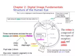
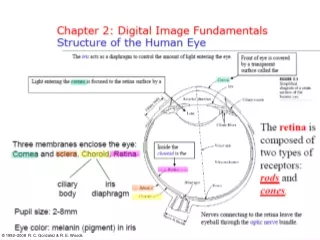
Monochromatic (achromatic) light: Light that is void of color - Attribute: Intensity (amount) . - Gray level is used to describe monochromatic intensity. Chromatic light: To describe it, three quantities are used: - Radiance: The total amount of energy that flows from the light source (measured in Watts). - Luminance: The amount of energy an observer perceives from a light source (measured in lumens). - Brightness: A subjective descriptor of light perception that is impossible to measure (key factor in describing color sensation) Definitions
Image Sensing & Acquisition How to transform illumination energy into digital images using sensing devices
Image Sensing & Acquisition • Image Acquisition using single sensor
Image Sensing & Acquisition • Image Acquisition using Sensor Strips scanners
Image Sensing & Acquisition • Image Acquisition using Sensor Array
White Light Colours Absorbed Green Light Reflected Light • The colours that we perceive are determined by the nature of the light reflected from an object • For example, if white light is shone onto a green object most wavelengths are absorbed, while green light is reflected from the object
Simple Image Formation Model • Simple image formation • f(x,y) = i(x,y)r(x,y) • i(x,y): illumination (determined by ill. Source) • 0 < i(x,y) < ∞ • i(x,y) = 90,000 lm/m2 (clear day), 0.1lm/m2 (evening) • i(x,y) = 10,000 lm/m2 (cloudy day), • r(x,y) reflectance (determined by imaged object) • 0 < r(x,y) < 1 • 0.01 for black velvet • 0.65 for stainless steel • In real situation • Lmin≤ L=f(x,y) ≤ Lmax • Lmin = imin * rmin • Lmax = imax * rmax • L : gray level
Image Sampling & quantization Continues image f(x,y) needs to be in digital form. Digitizing the coordinate values called sampling. Sampling should be in both coordinates and in amplitude. Image Sampling
Image Quantization Image Sampling & quantization Digitizing the Amplitude values called image quantization. Sampling limits established by no. of sensors, but quantization limits by color levels.
Image Sampling & quantization Digital Image Representation Each element called image element, picture element, or pixel
Image Sampling & quantization The notation (0,1), is used to signify the second sample along the first row, not the actual physical coordinates when the image was sampled
Image Sampling & quantization Consider an image which has : M * N : size of the image L : Number of discrete gray levels in this image L= 2k Where k is any positive integer The total number of bits needed to store this image b : b = M * N * K, If M = N, then b= N2 * K
Image Sampling & quantization The dynamic range is the ratio of the max (determined by saturation) measurable intensity to the min. (limited by noise) detectable intensity. Contrast is defined as the difference in intensity between the highest and the lowest intensity levels in an image.
Image Sampling & quantization • The dynamic range of an image can be described as: • High dynamic range: • Gray levels span a significant portion of the gray scale. • Low dynamic range: • Dull, washed out gray look.
Spatial resolution: - # of samples per unit length or area. - Lines and distance: Line pairs per unit distance. • Gray level resolution: - Number of bits per pixel. - Usually 8 bits. - Color image has 3 image planes to yield 8 x 3 = 24 bits/pixel. - Too few levels may cause false contour. Image Sampling & quantization
Image Sampling & quantization The subsampling was accomplished by deleting the appropriate number of rows and columns from the original image. Spatial Image Resolutions No. of gray levels (K) is constant(8-bits images). No. of samples (N) is reduced (No. of sensors)
Image Sampling & quantization Comparison between all image sizes
Image Sampling & quantization Gray Level Image Resolutions No. of samples (N) is constant, but gray levels (K) decreases. (false contouring)
Image Sampling & quantization What is the effect of changing N and K..? Little, Intermediate, and Large amount of details
Image Sampling & quantization Isopreference Curve
Image Interpolation • Interpolation is the process of using known data to estimate values at unknown locations. • Interpolation is a basic tool used in tasks such as zooming, shrinking, rotating, and geometric correction. • shrinking and zooming (resampling) • Zooming : requires two steps • Creation of a new pixel location • Assignment of a gray level to those new locations
Image Interpolation • Nearest neighbour interpolation (ex 500 x 500 image) • Laying an imaginary 750 x 750 grid over the original image • Shrink it so that it fits exactly over the original image • Spacing in the grid will be less than one pixel • Look for the closest pixel in the original image and assign its gray level to the new pixel in the grid. • Fast but produces checkerboard effect
Image Interpolation • Bilinear interpolation (four neighbours of point) • Let x, y a point in the zoomed image • v (x, y) a gray level assigned to it • v is given by • v (x, y) = ax + by + cxy +d • The coefficients are determined from the four equations using the four neighbours. • Bicubic interpolation (16 coefficeints) • Better job of preserving finer details • Standard in commercial image editing programs
Relationship Between Pixels 1- Neighbors of a Pixel: The 4- neighbors of pixel p are: N4(p) The 4- diagonal neighbors are: ND(p) The 8-neighbors are : N8(p)
Relationship Between Pixels • Adjacency of Pixels:- • Let V be the set of intensity used to define adjacency; e.g. V={1} if we are referring to adjacency of pixels with value 1 in a binary image with 0 and 1. • In a gray-scale image, for the adjacency of pixels with a range of intensity values of , say, 100 to 120, it follows that V={100,101,102,…,120}. • We consider three types of adjacency :
Adjacency • 4- adjacency • Two pixels p and q with values from V are 4- adjacency if q is in the set N4(p) .
Adjacency • 8- adjacency • Two pixels p and q with values from V are 8- adjacency if q is in the set N8(p) . • m- adjacency (mixed adjacency) • Two pixels p and q with values from V are m- adjacency if • (i) q is in N4(p) , or • (ii) q is in ND( p) and N4( p) ∩ N4 (q) is empty
Path • A (digital) path(or curve) from pixel p at (x,y) to pixel q at (s,t) is a sequence of distinct pixels with coordinates • (x0,y0), (x1,y1), …,, (xn,yn) • where (x0,y0) =(x,y), (xn,yn)=(s,t), and pixel (xi,yi) and (xi-1,yi-1) are adjacent for 1≤ i ≤ n • n is the length of the path • If (x0,y0) =(xn,yn), the path is a closed path • The path can be defined 4-,8-,m-paths depending on adjacency type
Connectivity • Let S be a subset of pixels in an image. • Two pixels p and q are said to be connected in S if there exists a path between them consisting entirely of pixels in S • For any pixel p in S, the set of pixels that are connected to it in S is called a connected component of S. • If it only has one connected component, then set S is called a connected set.
Region • Let R be a subset of pixels in an image. We call R a region of the image if R is a connected set • Two regions are said to be adjacent if their union forms a connected set. • Ri, Rj are adjacent in 8-adjacency sense. • They are not adjacent in 4-adjacency sense.
Boundary • Suppose that an image contains K disjoint regions, Rk, k = 1,2 ,...,k, none of which touches the image border. • Let Ru be the union of all the K regions, and let (Ru)c denote its complement. • We call the points in Ru the foreground, and all the points in (Ru)c the background of the image. • The inner boundary (border or contour) of a region R is the set of points that are adjacent to the points in the complement of R. i.e set of pixels in the region that have at least one background neighbour.
Boundary The point circle is not member of the border of the 1-valued region if 4-connectivity is used. As a rule, adjacency between points in a region and its background is defined in terms of 8-connectivity.
Boundary • The outer border corresponds to the border in the background. • This definition to guarantee the existence of a closed path
for pixel p, q and z with coordinates (x,y), (s,t) and (u,v) respectively, D is a distance function or metric if (a) D(p,q) ≥ 0 ; D(p,q) = 0 iff D=q (b) D(p,q) = D(q,p) (c) D(p,z) ≤ D(p,q) + D(q,z) Distance Measures
Distance Measures 1- The Euclidean distance between p and q is defined as:
Distance Measures 2- The D4 distance (city-block distance) between p and q is defined as:
Distance Measures 3- The D8 distance (chessboard distance) between p and q is defined as
Distance Measures 4- The Dm distance: the shortest m-path between the points.
Array Versus Matrix Operations • Array product • See matrix multiplication
Linear versus Nonlinear Operations • Consider general operator H • H is said to be a linear operator if • Assume sum operator
Linear versus Nonlinear Operations • Let a1 = 1 , a2 =-1
Arithmetic Operations • Carried out between corresponding pixel pairs • Same size of arrays • Let g(x,y) denote a corrupted image formed by the addition of noise η(x,y), to a noiseless image f(x,y); • g(x,y) = f(x,y) + η(x,y) • where the assumption is that at every pair of coordinates (x,y) the noise is uncorrelated and has a zero average.
Arithmetic Operations • If the noise satisfies the constrains just stated, then an image g(x,y) is formed by averaging K different noisy images, • As K increases the variability of the pixels at each location decreases.