Download
1 / 41
410 likes | 523 Views
Power calculation for QTL association (discrete and quantitative traits). Shaun Purcell & Pak Sham Advanced Workshop Boulder, CO, 2003. High Low A n 1 n 2 a n 3 n 4. Aff UnAff A n 1 n 2 a n 3 n 4. Tr UnTr A n 1 n 2 a n 3 n 4.

E N D
Power calculation for QTL association(discrete and quantitative traits) Shaun Purcell & Pak Sham Advanced Workshop Boulder, CO, 2003
High Low A n1 n2 a n3 n4 Aff UnAff A n1 n2 a n3 n4 Tr UnTr A n1 n2 a n3 n4 Tr UnTr A n1 n2 a n3 n4 Discrete Threshold Variance components Case-control Case-control • Quantitative TDT TDT
Discrete trait calculation • p Frequency of high-risk allele • K Prevalence of disease • RAA Genotypic relative risk for AA genotype • RAa Genotypic relative risk for Aa genotype • N, , Sample size, Type I & II error rate
Risk is P(D|G) • gAA = RAAgaagAa = RAagaa • K = p2gAA + 2pqgAa + q2gaa • gaa = K / ( p2 RAA + 2pq RAa + q2 ) • Odds ratios (e.g. for AA genotype) = gAA / (1- gAA ) • gaa / (1- gaa )
Need to calculate P(G|D) • Expected proportion d of genotypes in cases • dAA = gAA p2 / (gAAp2 + gAa2pq + gaaq2 ) • dAa = gAa2pq / (gAAp2 + gAa2pq + gaaq2 ) • daa = gaaq2 / (gAAp2 + gAa2pq + gaaq2 ) • Expected number of A alleles for cases • 2NCase ( dAA + dAa / 2 ) • Expected proportion c of genotypes in controls • cAA = (1-gAA) p2 / ( (1-gAA) p2 + (1-gAa) 2pq + (1-gaa) q2 )
Full contingency table • “A” allele “a” allele • Case 2NCase ( dAA + dAa / 2 ) 2NCase ( daa + dAa / 2 ) • Control 2NControl ( cAA + cAa / 2 ) 2NControl ( caa + cAa / 2 )
Threshold selection • Genotype AA Aa aa • Frequency q2 2pq p2 • Trait mean -a d a • Trait variance 2 2 2
P(X) = GP(X|G)P(G) P(X) Aa AA aa X
P(G|X<T) = P(X<T|G)P(G) / P(X<T) P(X) Nb. the cumulative standard normal distribution gives the area under the curve, P(X < T) Aa T AA X
A a Mpm1 + δ qm1 - δ mpm2 – δ qm2 + δ δ = D’ × DMAX DMAX = min{pm2 , qm1} Incomplete LD • Effect of incomplete LD between QTL and marker Note that linkage disequilibrium will depend on both D’ and QTL & marker allele frequencies
Incomplete LD • Consider genotypic risks at marker: • P(D|MM) = [ (pm1+ δ)2 P(D|AA) • + 2(pm1+ δ)(qm1- δ) P(D|Aa) • + (qm1- δ)2 P(D|aa) ] • / m12 • Calculation proceeds as before, but at the marker Haplo. Geno. AM/AM AAMM AM/aM or aM/AM AaMM aM/aM aaMM MM
Discrete TDT calculation • Calculate probability of parental mating type given affected offspring • Calculate probability of offspring genotype given parental mating type and affected • Calculate overall probability of heterozygous parents transmitting allele A as opposed to a • Calculate TDT test statistic, power
Fulker association model The genotypic score (1,0,-1) for sibling i is decomposed into between and within components: deviation from sibship genotypic mean sibship genotypic mean
NCPs of B and W tests Approximation for between test Approximation for within test Sham et al (2000) AJHG 66
Practical Exercise • Calculation of power for simple case-control study. • DATA : frequency of risk factor in 30 cases and 30 controls • TEST : 2-by-2 contingency table : chi-squared • (1 degree of freedom)
Step 1 : determine expected chi-squared • Hypothetical risk factor frequencies • Case Control • A allele present 20 10 • A allele absent 10 20 Chi-squared statistic = 6.666
Step 2. Determine the critical value for a given type I error rate, - inverse central chi-squared distribution P(T) Critical value T
Step 3. Determine the power for a given critical value and non-centrality parameter - non-central chi-squared distribution P(T) Critical value T
2. Calculate power (Non-central 2) Crit. value Expected NCP Calculating Power 1. Calculate critical value (Inverse central 2) Alpha 0 (under the null)
3.84146 6.63489 10.82754 • http://workshop.colorado.edu/~pshaun/gpc/pdf.html • df = 1 , NCP = 0 • X • 0.05 • 0.01 • 0.001
0.73 0.50 0.24 Determining power • df = 1 , NCP = 6.666 • X Power • 0.05 3.84146 • 0.01 6.6349 • 0.001 10.827
1. Planning a study • Candidate gene study • A disease occurs in 2% of the population • Assume multiplicative model • genotype risk ratio Aa = 2 • genotype risk ratio AA = 4 • 100 cases, 100 controls • What if the risk allele is rare vs common?
2. Interpreting a negative result • Negative candidate gene TDT study, • 82 affected offspring trios • “affection” = scoring >2 SD above mean • candidate gene SNP allele frequency 0.25 • Desired 80% power, 5% type I error rate • What is the minimum detectable QTL variance (assume additivity)?
Planning a study • p N cases (=N controls) • 0.01 1144 • 0.05 247 • 0.2 83 • 0.5 66 • 0.8 126 • 0.95 465 • 0.99 2286
Interpreting a negative result • QTL Power • 0.00 0.05 • 0.01 0.34 • 0.02 0.60 • 0.03 0.78 • 0.04 0.88 • 0.05 0.94
Exploring power of association using GPC • Linkage versus association • difference in required sample sizes for specific QTL size • TDT versus case-control • difference in efficiency? • Quantitative versus binary traits • loss of power from artificial dichotomisation?
Linkage versus association QTL linkage: 500 sib pairs, r=0.5 QTL association: 1000 individuals
Case-control versus TDT p = 0.1; RAA = RAa = 2
Quantitative versus discrete K=0.05 K=0.2 K=0.5 To investigate: use threshold-based association Fixed QTL effect (additive, 5%, p=0.5) 500 individuals For prevalence K Group 1 has N and T Group 2 has N and T
Quantitative versus discrete • K T (SD) • 0.01 2.326 • 0.05 1.645 • 0.10 1.282 • 0.20 0.842 • 0.25 0.674 • 0.50 0.000
Incomplete LD • what is the impact of D’ values less than 1? • does allele frequency affect the power of the test? • (using discrete case-control calculator) • Family-based VC association: between and within tests • what is the impact of sibship size? sibling correlation? • (using QTL VC association calculator)
Incomplete LD • Case-control for discrete traits • Disease K = 0.1 • QTL RAA = RAa = 2 p = 0.05 • Marker1 m = 0.05 D’ = { 1, 0.8, 0.6, 0.4, 0.2, 0} • Marker2 m = 0.25 D’ = { 1, 0.8, 0.6, 0.4, 0.2, 0} • Sample 250 cases, 250 controls
Incomplete LD • Genotypic risk at marker1 (left) and marker2 (right) as a function of D’
Incomplete LD • Expected likelihood ratio test as a function of D’
Family-based association • Sibship type • 1200 individuals, 600 pairs, 400 trios, 300 quads • Sibling correlation • r = 0.2, 0.5, 0.8 • QTL (diallelic, equal allele frequency) • 2%, 10% of trait variance
Family-based association • NCP proportional to variance explained • Between test • ↓ with ↑ sibship size and ↑ sibling correlation • Within test • 0 for s=1, ↑ with ↑ sibship size and ↑ sibling correlation
GPC • Usual URL for GPC • http://statgen.iop.kcl.ac.uk/gpc/ Purcell S, Cherny SS, Sham PC. (2003) Genetic Power Calculator: design of linkage and association genetic mapping studies of complex traits. Bioinformatics, 19(1):149-50