Download
1 / 26
310 likes | 546 Views
QTL mapping. Simple Mendelian traits are caused by a single locus, and come in the ‘ all-or-none ’ flavor. A Quantitative Trait is one in which many loci contribute. The phenotype can therefore vary in a ‘ quantitative ’ manner. Ades 2008, NHGRI. Modified from Mike White slides, 2010.

E N D
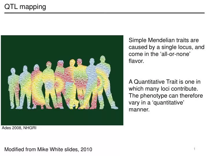
QTL mapping Simple Mendelian traits are caused by a single locus, and come in the ‘all-or-none’ flavor. A Quantitative Trait is one in which many loci contribute. The phenotype can therefore vary in a ‘quantitative’ manner. Ades 2008, NHGRI Modified from Mike White slides, 2010
Goals of QTL mapping • To identify the loci that contribute to phenotypic variation • Cross two parents with extreme phenotypes • Score the progeny for the phenotype • Genotype the progeny at markers across the genome • Associate the observed phenotypic variation with the underlying genetic variation • Ultimate goal: identify causal polymorphisms that explain the phenotypic variation Ades 2008, NHGRI Modified from Mike White slides, 2010
Backcross Phenotype: Drug tolerance 80% 20% viability Usually have at least 100 individuals Broman and Sen 2009
Intercross Phenotype: Drug tolerance 80% 20% viability Broman and Sen 2009
Backcross vs. Intercross • An intercross recovers all three possible genotypes (AA, BB, AB). This allows detection of dominance with both alleles and provides estimates of the degree of dominance. • A backcross has more power to detect QTL with fewer individuals. • A backcross may be the only possible scheme when crossing two different species.
Genetic map: specific markersspaced across the genome • Markers can be: • SNPs at particular loci • Variable-length repeats • e.g. ALU repeats • ALL polymorphisms • (if have whole genomes) Ideally, markers should be spaced every 10-20 cM and span the whole genome
Test which markers correlate with the phenotype • Missing Data Problem • Use marker data to infer intervening genotypes • 2. Model Selection Problem • How do the QTL across the genome combine with the covariates to generate the phenotype? Broman and Sen 2009
Test which markers correlate with the phenotype Marker regression: simple T-test (or ANOVA) at each marker Marker 1: no QTL Marker 2: significant QTL (population means are different)
Marker regression Advantages: • Simple test – standard T-test/ANOVA • Covariates (e.g. Gender, Environment) are easy to incorporate • No genetic map necessary, since test is done separately on each marker Disadvantages: • Any individuals with missing marker data must be omitted from analysis • Does not effectively consider positions between markers • Does not test for genetic interactions (e.g. epistasis) • The effect size of the QTL (i.e. power to detect QTL) is reduced by incomplete • linkage to the marker • Difficult to pinpoint QTL position, since only the marker positions are considered
Interval mapping • Lander and Botstein 1989 • In addition to examining phenotype-genotype associations at markers, look for associations between makers by inferring the genotype A A A A Q • The methods for calculating genotype probabilities between markers typically use hidden Markov models to account for additional factors, such as genotyping errors
Interval mapping Broman and Sen 2009
Interval mapping Advantages: • Takes account of missing genotype information – all individuals are included • Can scan for QTL at locations in between markers • QTL effects are better estimated Disadvantages: • More computation time required • Still only a single-QTL model – cannot separate linked QTL or examine for interactions among QTL
LOD scores • Measure of the strength of evidence for the presence of a QTL • at each marker location LOD(λ) = log10 likelihood ratio comparing the hypothesis of a QTL at position λ versus that of no QTL } { Pr(y|QTL at λ, µAAλ,µABλ,σλ) log10 Pr(y|no QTL, µ,σ) LOD 3 means that the TOP model is 103 times more likely than the BOTTOM model Phenotype
LOD curves How do you know which peaks are really significant?
LOD threshold • Consider the null hypothesis that there are no QTLs genome-wide one location genome-wide Randomize the phenotype labels on the relative to the genotypes Conduct interval mapping and determine what the maximum LOD score is genome-wide Repeat a large number of times (1000-10,000) to generate a null distribution of maximum LOD scores Broman and Sen 2009
LOD threshold • 1000 permutations • 10% ‘Genome-wide Error Rate’ = LOD 3.19 • (means that at this LOD cutoff 10% of peaks could be random chance) • 5% GWER = LOD 3.52 • Boundary of the peak is often taken as points that cross (Max LOD – 1.5) (or - 1.8 for an intercross) • Often these regions are very large & encompass many (hundreds) of genes
Lessons from QTL mapping studies about Genetic Architecture * Often have a few big effect QTL and many small modifier QTL with small effects on the phenotype need lots of power (good phenotypic measurements and many individuals) to detect QTLs with small effects * Recombination in F2’s can reveal negative effects segregating in the parents e.g. can find resistant-parent allele associated with sensitivity MacKay review: often have loci with complementary effects found nearby * Effects of an allele can be context dependent Environment-specific effects: Gene x Environment (GxE) interactions Genomic context: epistatic (i.e. gene-gene) interactions are likely very common … but difficult to detect
An alternative approach: Genome Wide Association Studies (GWAS) Here the phenotypes and genotypes come from many different individuals from a population • Identify SNPs that are significantly associated with the trait • across a bunch of individuals
An alternative approach: Genome Wide Association Studies (GWAS) across many individuals Genotypes for 65 strains Phenotypes for 65 strains Population Structure Phylogenetic Relatedness Random Error Random Error Strains Typically use a mixed linear model to test for significance Phenotypic variance y = μ + a + other stuff + Error Additive Genetic Effects across all involved genes Phenotypic mean
Identify SNPs that are significantly associated with the trait Phenotype AA TT Genotype
A very important control for both types of mapping: controlling for covariates Sometimes a SNP can appear correlated with phenotypic variation … but it can be due to some other feature that co-varies with the SNP and the phenotype The clearest example: population structure Other examples: - gender of the individuals - shared environments for subgroups - an example from our yeast studies: ploidy differences when some F2s are haploid and some are diploid
Example: S. cerevisiae strains (Liti et al. 2009) Vineyard strains Oak strains Phenotype TT AA Genotype
Mixed linear model identifies SNPs with a significant p-value. Often plot the –log(p) across the genome (Manhattan plot) Again, the p-value cutoff comes from permutations (randomize the strain-phenotype labels and perform mapping on randomized data 10,000 times)
How to find the causative SNP/polymorphism in giant regions? Often very challenging to find which SNP(s) or polymorphisms (copy-number differences, rearrangements, etc) are causal Some strategies people use: - Look at what’s known about the genes in the peak CAUTION: very easy to get led by what ‘seems likely’ - Look at signatures of selection within the population e.g. differences in FST - Look for derived alleles - Look for coding changes, genes in the region with severe expression differences - Combine with other data e.g. other mapping studies (QTL + GWAS), genomic datasets