Download
1 / 75
810 likes | 1.18k Views
Chapter 8 Quantitative Genetics. Traits such as cystic fibrosis or flower color in peas produce distinct phenotypes that are readily distinguished. Such discrete traits , which are determined by a single gene, are the minority in nature.

E N D
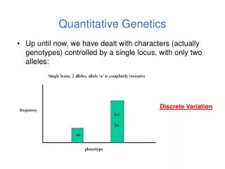
Chapter 8 Quantitative Genetics • Traits such as cystic fibrosis or flower color in peas produce distinct phenotypes that are readily distinguished. • Such discrete traits, which are determined by a single gene, are the minority in nature. • Most traits are determined by the effects of multiple genes.
Continuous Variation • Traits determined by many genes show continuousvariation. • Examples in humans include height, intelligence, athletic ability, skin color. • Beak depth in Darwin’s finches and beak length in soapberry bugs also show continuous variation.
Quantitative Traits • For continuous traits we cannot assign individuals to discrete categories. Instead we must measure them. • Therefore, characters with continuously distributed phenotypes are called quantitative traits.
Quantitative Traits • Quantitative traits determined by influence of (1) genes and (2) environment.
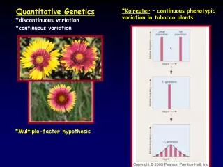
East’s 1916 work on quantitative traits • In early 20th century debate over whether Mendelian genetics could explain continuous traits. • Edward East (1916) showed it could. • Studied longflower tobacco (Nicotianalongiflora)
East’s 1916 work on quantitative traits • East studied corolla length (petal part of flower) in tobacco. • Crossed pure breeding short and long corolla individuals to produce F1 generation. Crossed F1’s to create F2 generation.
East’s 1916 work on quantitative traits • Using Mendelian genetics we can predict expected character distributions if character determined by one gene, two genes, or more etc. • (You need to understand how to do Punnett Squares)
East’s 1916 work on quantitative traits • Depending on number of genes, models predict different numbers of phenotypes. • One gene: 3 phenotypes • Two genes: 5 phenotypes • Six genes: 13 phenotypes. Continuous distribution.
East’s 1916 work on quantitative traits • How do we decide if a quantitative trait is under the control of many genes? • In one- and two-locus models many F2 plants have phenotypes like the parental strains. • Not so with 6-locus model. Just 1 in 4,096 individuals will have the genotype aabbccddeeff.
East’s 1916 work on quantitative traits • But, if Mendelian model works you should be able to recover the parental phenotypes through selective breeding. • East selectively bred for both short and long corollas. By generation 5 most plants had corolla lengths within the range of the original parents.
East’s 1916 work on quantitative traits • Plants in F5 generation of course were not exactly the same size as their ancestors even though they were genetically identical. • Why?
East’s 1916 work on quantitative traits • Environmental effects. • Because of environmental differences genetically identical organisms may differ greatly in phenotype.
Genetically identical plants grown at different elevations differ enormously (Clausen et al. 1948)
Measuring Heritable Variation • A person’s height is determined by their genes operating within their environment. • Heritability measures what fraction of variation in height is due to variation in genes and what fraction is due to variation in environment.
Measuring Heritable Variation • Heritability measured based on population data. • Total variation in trait is phenotypic variation Vp. • Variation among individuals due to their genes is genetic variation Vg • Variation among individuals due to their environment is environmental variation Ve.
Measuring Heritable Variation • Heritability = Vg/Vp • Heritability = Vg/Vg+Ve • This is broad-sense heritability. Heritability always a number between 0 and 1.
Estimating heritability from parents and offspring • If variation among individuals is due to variation in genes then offspring will resemble their parents. • Can assess relationship using scatter plots.
Estimating heritability from parents and offspring • Plot midparent value (average of the two parents) against offspring value.
Estimating heritability from parents and offspring • If offspring don’t resemble parents then best fit line has a slope of approximately zero. • Slope of zero indicates most variation in individuals due to variation in environments.
Estimating heritability from parents and offspring • If offspring strongly resemble parents then best fit line will be close to 1.
Estimating heritability from parents and offspring • Most traits in most populations fall somewhere in the middle with offspring showing moderate resemblance to parents.
Estimating heritability from parents and offspring • Slope of best fit line is between 0 and 1. • Slope represents narrow-sense heritability (h2).
Narrow-sense heritability • Narrow-sense heritability distinguishes between two components of genetic variation: • Va additive genetic variation: variation due to additive effects of genes. • Vd dominance genetic variation: variation due to gene interactions such as dominance.
Narrow-sense heritability • h2 = Va/(Va + Vd + Ve)
Narrow-sense heritability • When estimating heritability important to remember parents and offspring share environment. • Need to make sure there is no correlation between environments experienced by parents and offspring. Requires cross-fostering experiments.
Smith and Dhondt (1980) • Smith and Dhondt (1980) studied heritability of beak size in Song Sparrows. • Moved eggs and young to nests of foster parents. Compared chicks’ beak dimensions to parents and foster parents.
Smith and Dhondt (1980) • Smith and Dhondt estimated heritability of bill depth about 0.98.
Estimating heritability from twins • Monozygotic twins are genetically identical dizygotic are not. • Studies of twins can be used to assess relative contributions of genes and environment to traits.
McClearn et al.’s (1997) twin study • McClearn et al. (1997) used twin study to assess heritability of general cognitive ability. • Studied 110 pairs monozygotic and 130 pairs dizygotic twins in Sweden.
McClearn et al.’s (1997) twin study • All twins at least 80 years old, so plenty of time for environment to exert its influence. • However, monozygotic twins resembled each other much more than dizygotic. • Estimated heritability of trait at about 0.62.
Measuring differences in survival and reproduction • Heritable variation in quantitative traits is essential to Darwinian natural selection. • Also essential is that there are differences in survival and reproductive success among individuals. Need to be able to measure this.
Measuring differences in survival and reproduction • Need to be able to quantify difference between winners and losers in trait of interest. This is strength of selection.
Measuring differences in survival and reproduction • If some animals in a population breed and others don’t and you compare mean values of some trait (say mass) for the breeders and the whole population, the difference between them (and one measure of the strength of selection) is the selection differential (S).
Measuring differences in survival and reproduction • Another measure of the strength of selection is the selection gradient. • Assign absolute fitnesses to members of population. • Convert absolute fitnesses to relative fitnesses (absolute fitness/mean fitness). • Make scatterplot of relative fitness against trait if interest. Slope of best-fit line is selection gradient.
Selection gradient • Selection gradient = (selection differential/variance of trait of interest.)
Evolutionary response to selection • Knowing heritability and selection differential can predict evolutionary response to selection (R). • Given by formula: R=h2S • R is predicted response to selection, h2 is heritability, S is selection differential.