Download
1 / 37
370 likes | 375 Views
This study explores the reconstruction of sea-level changes during the Holocene along the mid-Atlantic coast of the USA. The study uses a standardized approach to calculate relative sea-level (RSL) changes, taking into account isostatic changes, minimal meltwater input, and negligible tectonic effects. The findings show that RSL rapidly rises during the early and mid-Holocene, with no evidence of being above present levels. There is an increase in the rate of RSL rise during the 20th century compared to the late Holocene. The study acknowledges the contribution of various researchers in compiling the sea-level database and developing the methodology.

E N D
Holocene relative sea-level changes of the mid Atlantic coast of the USA Ben Horton Simon Engelhart Dick Peltier Tor Törnqvist David Hill
Reconstruction of sea level The sea-level equation: rsl(,) = eus()+iso(,)+tect(,)+local(,)
Employ a standardized approach • Location: the geographical coordinates of the sample site • Age: calibrated years BP using IntCal04 or Marine04 (0-26 cal kyrs BP) • Elevation: To measure RSL change, it is necessary to establish the relationship of the sample to a tide level (indicative meaning)
Indicative meaning (modern) Indicative meaning defines the relationship between a sea-level indicator and a reference water level (e.g. mean tide level)
Indicative meaning (application to the past) RSL is calculated by subtracting the reference water level from the elevation of the dated sample (B, C). Where deposition is in a freshwater or marine environments, the sample is classified as a “limiting date” (A, D).
RSL change during the late Holocene rsl(,) = eus()+iso(,)+tect(,)+local(,) • Minimal meltwater input (eus) from 4 ka BP to 1900AD • Compaction errors minimized and tidal range change negligible in the last 4ka (local) • Negligible tectonic effects tect(,) rsl(,) ~ iso(,) • Last 4 ka is an indicator of isostatic adjustment primarilydue to the Laurentide Ice Sheet (iso) • Compare with tide gauge records of 20th century RSL
Late Holocene vs. 20th century Increase in rate of RSLR of 1.8 ± 0.2 mm/yr
Summary • >650 sea level data points • No data for Georgia to Florida and less than 10% of index points older than 6ka BP • RSL rapidly rises during the early and mid Holocene with no evidence of being above present • Increase 20th century and late Holocene RSLR is 1.8 ± 0.2 mm/yr. BUT this is not uniform; increases from north to south
Acknowledgments Torbjörn Törnqvist (Co-PI) for the advancement of an appropriate methodology for compiling the sea-level database Dick Peltier (Co-PI) for GIA predictions of sea-level and paleobathymetries David Hill (Co-PI) for tidal modeling Simon Engelhart (graduate) for collection and validation of sea-level data Ian Shennan, Orson van de Plassche, Bruce Douglas, Stephen Griffiths, Rob Theiler (steering committee) for help and much advice All the sea-level researchers who provided both published and unpublished data to this project and lent their expertise on the subject on numerous occasions.
Holocene tidal range change in the mid Atlantic • Tidal range (MHHW – MLLW) largely follows the trends in M2, the largest constituent • Even at 5kybp, only small changes noticed • Dramatic amplification occurs at 8 to 9K
ICE 5G and ICE 6G • Large effect on predictions Northeastern Atlantic • Little change in mid or southern Atlantic VM5a includes a 60 km thick perfectly elastic upper layer. Upper mantle viscosity of 0.5 * 1021 Pa s Peltier and Drummond, 2008, GRL, 35; Peltier et al., in review, PNAS
Old vs New • Increased number (>650 data points) compared to Peltier (1996) • Understanding of the indicative meaning • Elevation errors • No assessment of compaction or tidal range change • Significant implication for GIA model