Download

1 / 46
460 likes | 572 Views
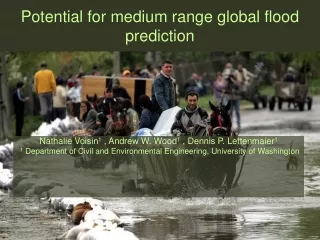
Global Flood and Drought Prediction. Nathalie Voisin and Dennis P. Lettenmaier Department of Civil and Environmental Engineering University of Washington Seattle, USA. www.ektopia.co.uk/ektopia/ images/parisflood.jpg. Outline. Background and Objective

E N D
Global Flood and Drought Prediction Nathalie Voisin and Dennis P. Lettenmaier Department of Civil and Environmental Engineering University of Washington Seattle, USA www.ektopia.co.uk/ektopia/ images/parisflood.jpg
Outline • Background and Objective • Data and models …Or why I think GCM met data are more appropriate for global streamflow forecasting for now • Toward developing global hydrology forecast capability • Approach • Data Processing : bias correction and downscaling of the forecasts • Preliminary results: Evaluation of the bias correction and the downscaling on two specific events • Future work
Need for flood prediction globally? www.dartmouth.edu/~floods, Dartmouth Flood Observatory
Global Floods and Droughts • Floods • $50-60 billion USD /year, worldwide ( United Nations University) • 520+ million people impacted per year worldwide • Estimates of up to 25,000 annual deaths Mostly in developing countries; Mozambique in 2000 and 2001, Vietnam and others (Mekong) in 2000. • Droughts • 1988 US Drought: $40 billion (1988 drought: NCDC ) • Famine in many countries: 200,000 people killed in Ethiopiain 1973-74 Source: United Nations University, http://update.unu.edu/archive/issue32_2.htm http://www.unu.edu/env/govern/ElNIno/CountryReports/inside/ethopia/Executive%20Summary/Executive%20Summary-txt.html 1988 drought: NCDC : http://lwf.ncdc.noaa.gov/oa/reports/billionz.html
Objective Predict streamflow and associated hydrologic variables, soil moisture, runoff, evaporation and snow water equivalent : 1. At a global scale • Spatial consistency • To cover ungauged or poorly gauged basins 2. Time scales: • Short term for floods • Seasonal (or longer) for drought 3. Freely disseminate information for agriculture, energy, food security ,and protection of life and property
Meteorological Data - Surface observations: Uneven global coverage Various attempts to grid globally We use Adam et al. (2006) 1979-1999 (0.5 degrees) and ERA-40 - Precipitation derived from satellite: Various products available, mostly either passive microwave and/or infra-red Issue with climatology and consistency ( especially important for seasonal prediction) - Climate Models: ECMWF and NCEP Re-analysis products, for at least 25 years Ensemble forecast products Quasi all or all required input data for our hydrologic model available
Meteorological Data - Comparison Precip Comparison of 1997-1999 monthly basin averages Runoff Evap Soil Moist SWE …Or why I think GCM met data are more appropriate for global streamflow forecasting for now
Meteorological Data - Comparison Precip Runoff Evap Soil Moist SWE …Or why I think GCM met data are more appropriate for global streamflow forecasting for now
Meteorological Data - Comparison Precip Runoff Evap Soil Moist SWE …Or why I think GCM met data are more appropriate for global streamflow forecasting for now
Meteorological Data In this paper , I conclude that : (1) Satellite precip need more “calibration” based on topography and in the ITCZ (2) Great hope that satellite will bring the “observed” small scale spatial variability available. Need longer climatology to be able to perform bias correction in order to correct for (1) (3) Missing data, issue in real time forecasting
The Hydrologic Model VIC - Already calibrated and validated at 2 degree resolution on over 26 basins worldwide(Nijjsen et al. 2001) • Calibrated and validated at 0.5 degree over the Arctic domain • Ongoing with UW and Princeton globally at 0.5 degree resolution • Routing at 0.5 degree derived from SRTM30 and from the manually corrected global direction file from Doell and Lehner (2002)
INITIAL STATE Forecast System Schematic * soil moisture snowpack streamflow, soil moisture, snow water equivalent, runoff local scale (1/2 degree) weather inputs Hydrologic forecast simulation Hydrologic model spin up Ensemble Reforecasts NCEP Reforecasts (Hamill 2006), bias corrected w/r to ERA40 and downscaled w/r to Adam et al. (2006) observations ( NCEP GFS, ECMWF ESP) ECMWF ERA40 (or Analysis) Later on: CMORPH, MODIS, AMSR-E, others SNOTELUpdate NOWCASTS SEASONAL FORECASTS (drought) Several years back Month 0 SHORT TERM FORECASTS (flood) * Similar experimental procedure as used by Wood et al (2005) West-wide seasonal hydrologic forecast system
Spin Up • ECMWF ERA40 reanalysis for retrospective forecasting • Assume ERA40 is the truth • Later use ECMWF analysis field, bias corrected to match ERA40 characteristics
The Meteorological Forecasts Retrospective forecasting: Reforecasts • Tom Hamill (2006) NOAA • NCEP-MRF, 1998 version • 1979-present • 15-day forecasts issued daily • 15 member ensemble forecast • 2.5 degree resolution (Near) Real Time forecasting: ECMWF and/or NCEP (future)
Data processing The climatology statistics to be conserved in the forecasts are : - the frequency of occurrence of rain- the peaks - accumulated amounts (mean)
Data processing: Bias Correction Non-exceedance probability plots (MRF in green, ERA40 in black ) Systematic Bias Occurrence of Precipitation
Data processing: Bias Correction Systematic bias Using quantile-quantile mapping technique Occurrence of Precipitation
Data processing: Downscaling • Inverse square distance interpolation from 2.5 down to 0.5 degree resolution • Integration of observation based spatial variability at 0.5 degree: • Use observations based Adam et al. (2006) global dataset (0.5 degree resolution) • Shifting : • makes the Adam et al. average temperature field at 2.5 degree match ERA40, • Derive the temperature range for each 0.5 degree cell within the 2.5 degree cell • Scaling of the precipitation and the wind field so that the ratio Value(0.5)/Value(2.5) is conserved
Downscaling: observation based spatial variability at 0.5 degree: • Choose the year that will give the variability: • Choose randomly one single year (1979-1999) for all cells and all lead times • For retrospective forecasting, choose the year of the forecast. • Rainy and non rainy days records from Adam et al. 2006 (averaged to 2.5 degrees) dataset, are classified and saved for the month of the lead time: • RecordRain(cell, month of fcst) and RecordNonRain(cell, month of fcst) • Shitfing and/or scaling: • If Raining: select randomly a record in the RecordRain database, the record is conserved for the 4 variables. • Precip0.5=GFSbiascorrected,2.5 / Adam2.5(recordrain) * Adam0.5(recordrain) • Tavg0.5=GFSbiascorrected,2.5- Adam2.5(recordrain) + Adam0.5(recordrain) • Wind0.5=GFSbiascorrected,2.5 / Adam2.5(recordrain) * Adam0.5(recordrain) • Adjust Tmin and Tmax • DeltaTemp=TmaxAdam0.5(recordrain)-TminAdam0.5(recordrain) • Tmax0.5=Tavg0.5+1/2*DeltaTemp and Tmin0.5=Tavg0.5-1/2*DeltaTemp
Downscaling Adam et al. Random rainy day ( in the mth of fcst) Bias corrected GFS reforecast 2.5 degree 0.5 degree 2.5 degree Rain Scaling: Normalize the 0.5 degree spatial variability Shifting: Save the (Value0.5-Value2.5) No Rain Shifting of temperature and scaling of wind based on any Non Rainy day
Downscaling Notes: Sometimes, bias corrected GFS reforecast calls for rain but there is No rain in the Adam et al. dataset for the (randomly) selected year. In this case, the 2.5 degree cell is downscaled to 0.5 degree by inverse square distance interpolation. Tmin and Tmax are derived from a randomly selected record. If I was to select another year: • No guarantee that there is rain in a different year • The additional computing time and resources needed make it not worth doing it Downside of downscaling this way: any spatially large rain event (> 2.5 degree like fronts, etc) is not conserved because each 2.5 degree cell has an independently randomly selected RainRecord.
Retrospective Forecasting Interests: • Skills over different climate and basins • Skills for different type of floods: short term strong events ( fronts, extratropical or tropical storms) or sustained rain events ( monsoons). Events of interest: • Event 1: End of January 1995 : flood in the Meuse and Rhine basins (Europe) • Event 2: July 1997: flood in the Oder Basin (Europe) • Event 3: February 2000, flood in the Limpopo • Event 4: July-September 2000, flood in the Mekong
Retrospective Forecasting of Short Events • Event 1: End of January 1995 : flood in the Meuse and Rhine basins (Europe) • Event 3: February 2000, flood in the Limpopo
1995/01/20 Rhine – Effect of SMSC The Rhine Basin
1995/01/20 Rhine Precipitation w/o SMSC SMSC BC SMSC ERA40 LEAD 1 LEAD 2 LEAD 3
1995/01/20 Rhine Runoff w/o SMSC SMSC BC SMSC ERA40 LEAD 1 LEAD 2 LEAD 3
1995/01/20 Rhine PRECIPITATION W/o SMSC With SMSC ERA40
1995/01/20 Rhine RUNOFF W/o SMSC With SMSC ERA40
1995/01/20 Rhine Change in SWE W/o SMSC With SMSC ERA40
1995/01/20 Rhine Basin Avg Hydrologic Variables Prediction (ERA40 in red, GFS in black, NMC reanalysis in blue ) NO SMSC SMSC BC SMSCBC BC improves SWE (?) but does not do any miracle on missed precip peaks ( timing issue). Not significant improvement here though … SMSC gives a few “crazy” ensembles
2000/02/03 - Limpopo Limpopo
2000/02/03 Limpopo – Effect of SMSC PRECIPITATION W/o SMSC With SMSC ERA40
2000/02/03 Limpopo – Effect of SMSC Runoff W/o SMSC With SMSC ERA40
2000/02/03 Limpopo – CTRL PRECIPITATION without SMSC and BC GFS ens avg NMC rean ERA40
Conclusion • Bias correction implemented • Correction for occurrence of precip implemented • Downscaling implemented • Output variables: • By lead time: Precip, Runoff, Evap, Change in SWE, Change in Soil Moisture, Degree Days • 5 day accumulation: same • Time series: of basin average hydrologic variables and streamflow at selected stations
Conclusion on the Bias Correction The bias correction : • beneficial for ALL input variables (P, Tavg,Wind) • does not substitute for missed precipitation/temperature peaks/lows BUT the correction for the occurrence of rain correction should help ( not shown ) • brings consistency between the control run ( model or observations, or both) and the forecasts
Conclusion on the Downscaling • A few ensembles get crazy values ( should check the scaling factor) • The location of the front is not really respected, some information get lost ( maybe should interpolate linearly first, then shift or scale) • Adam et al. 2006 precipitation was disaggregated statistically in time. Should I expect real precipitation patterns (frontal shape, etc) within a 2.5 degree cell? Not appropriate for downscaling in a tropical storm event ; linear interpolation might be better in this case.
Future Work Retrospective forecasting: • Investigate more events and fix the remaining “bugs?”/make last improvements • Extend the retrospective forecasts: using archived ECMWF 10 day, monthly and seasonal forecasts • Predictions in forms of percentile and anomalies with respect to the climatology
Future Work Operational real time forecasting: • Once/Twice a week for short term forecasts • Use several climate model forecasts: • ECMWF 10 day forecast • ECMWF monthly forecast • ECMWF seasonal forecast • GFS 6-10 day forecast • Improvement of the initial conditions: e.g. assimilation of satellite soil moisture; snow
2000/02/03 Limpopo – Effect of SMSC Basin Avg Hydrologic Variables Prediction (ERA40 in red, GFS in black, NMC reanalysis in blue ) NO SMSC SMSC