Download
1 / 32
320 likes | 326 Views
Potential for medium range global flood prediction. Nathalie Voisin 1 , Andrew W. Wood 1 , Dennis P. Lettenmaier 1 1 Department of Civil and Environmental Engineering, University of Washington. Outline. Background and Objectives Description of the prediction scheme: The hydrology model

E N D
Potential for medium range global flood prediction Nathalie Voisin1 , Andrew W. Wood1 , Dennis P. Lettenmaier1 1 Department of Civil and Environmental Engineering, University of Washington
Outline • Background and Objectives • Description of the prediction scheme: • The hydrology model • The scheme • The bias correction • Use of satellite in the downscaling process of weather forecasts • Preliminary results for • Rhine Flood 1995 ( mostly rain, then snowmelt) • Limpopo flood 2000 (tropical storm)
Background Need for flood prediction globally? www.dartmouth.edu/~floods, Dartmouth Flood Observatory
Background Flood prediction systems exist • in developed Countries • What about developing countries? The potential for global flood prediction system exists • Global weather models : analysis and forecasts are available • Issues: scale?
Objectives Ultimate objective: to predict streamflow and associated hydrologic variables, soil moisture, runoff, evaporation and snow water equivalent : • At a global scale • Spatial consistency • Especially in ungauged or poorly gauged basins • medium-range time scale ( up to 2 weeks) This talk: to suggest a method to downscale global weather forecasts into a higher spatial resolution without any local information ( gauges or radar)
The global prediction scheme The hydrology model VIC - Semi-distributed model driven by a set of surface meteorological data ( precipitation, wind, solar radiation derived from Tmin and Tmax, etc) - Represents vegetation, has three soil layers with variable infiltration, non linear base flow.
The global prediction scheme The river routing model - Runoff and baseflow for each cell is then routed toward selected locations, following directions equivalent to channels. • Routing at 0.5 degree derived from the manually corrected global direction file from Döll and Lehner (2002) - Already calibrated and validated at 2 degree resolution over 26 basins worldwide(Nijssen et al. 2001)
The global prediction scheme (here in retrospective mode) Atmospheric inputs NCEP Reforecasts (Hamill et al. 2006)15 ensemble members – 15 day forecast – 2.5 degree (fixed GFS version of 1998) Daily ERA-40 downscaled to 0.5 degree using linear inverse distance square interpolation. Bias correctionat 2.5 degree, with respect to ERA-40 (Ensures consistency between spinup and the reforecasts) Downscalingfrom 2.5 to 0.5 degree using the Schaake Shuffle ( Clark et al. 2004) with higher spatial resolution satellite GPCP 1dd (Huffman et al. 2001) and TRMM 3B42 precipitations Hydrologic model spin up (0.5 degree global simulation) Hydrologic forecast simulation INITIAL STATE (0.5 degree global simulation: stream flow, soil moisture, SWE, runoff ) Several years back Nowcasts Medium range forecasts ( up to 2 weeks) Hydrology Model
Retrospective forecasting: Reforecasts • Hamill et al. (2006) NOAA • NCEP-MRF, 1998 version • 1979-present • 15-day forecasts issued daily • 15 member ensemble forecast • 2.5 degree resolution Near Real Time forecasting: ECMWF and/or NCEP analysis
The global prediction system The bias correction of GFS reforecasts (1) 1. Quantile-Quantile technique with respect to ERA-40 climatology • ERA-40 cdf based on a 9 day moving window, centered on the day of the forecast ( 9 * 23 values ) • GFS reforecast cdf for the 15 ensemble average, for each lead time, fixed 7 day window • Extreme values: low values fitted with Weibull distribution and high values fitted with Gumbel distribution Figure from Wood and Lettenmaier, 2004: A testbed for new seasonal hydrologic forecasting approaches in the western U.S.
The global prediction system The bias correction of GFS reforecasts (2) 2.Correction for daily intermittency ( with respect to ERA-40 climatology)
Use of satellite for downscaling forecasts Limpopo Basin, 2.5 degree grid South Africa, 2.5 degree grid Limpopo Basin, 0.5 degree grid
Use of satellite for downscaling forecasts Satellite Datasets • TRMM 3B42 • 50oS-50oN • 0.25 degree, 3 hourly, 2002-present • Use 2002-2006 ( to be updated yearly) • GPCP 1dd • Global, but used for 50oN-90oN and 50oS-90oS • 1 degree, daily, Oct 1996 – 3 months before present • Use 1997-2005 (to be updated yearly), interpolated to 0.5 degree using an inverse distance square interpolation.
Use of satellite for downscaling forecasts Simplified Schaake Schuffle (Clark et al. 2004) • to construct spatial patterns of precipitation within each 2.5 degree cell based on observations ( here, satellite) • For each 2.5 degree cell, for each lead time: • 15 satellite observations are randomly selected ( based on rain / no rain, specific to calendar month ) • for each ranked forecast ensemble member, it associates the corresponding ranked observation ( 15 ensemble members). → ensures that the selected highest observed precipitation event is assigned to the highest forecast GFS refcst, 2.5 deg, rank ith Satellite, 2.5 deg, rank ith
Use of satellite for downscaling forecasts TRMM 3B42 aggregated to daily and 2.5 degree resolution → resolution of the weather forecasts TRMM 3B42, 2.5 degree Jan 31st, 2001 TRMM 3B42 aggregated to daily and 0.5 degree resolution → resolution of the hydrologic model TRMM 3B42, 0.5 degree Jan 31st, 2001 →Need a downscaling method that inserts localized precipitation patterns (mm/day)
Use of satellite for downscaling forecasts Simplified Schaake Shuffle (2): • The corresponding observed value field at 0.5 degree resolution gives the spatial distribution of precipitation, but NOT the magnitude Here for one ensemble member, one lead time : = / Ratio of Satellite observations, 0.5 deg resolution Satellite, 0.5 deg, corresponding record to the 2.5 degree cells Satellite, 2.5 deg
Use of satellite for downscaling forecasts Dowscaling of precipitation characteristics: • Spatial distribution from satellite observations • Magnitude of the bias corrected GFS reforecasts • Consistency between spin up dataset and bias corrected downscaled forecasts Here for one ensemble member, one lead time : X = Bias corrected GFS refcst, 2.5 deg Ratio of satellite obs. 0.5 degree to 2.5 degree Bias corrected and downscaled (0.5 degree) GFS reforecast
Preliminary Results Rhine Flood, 1995 (Forecast of January 20th, 1995) • 5 day precipitation accumulation fields Bias correctedGFS Fcst. Ens. Avg, Downscaled ERA-40, simple interpol. GFS Det. Fcst., simple interpol. 1 to 5 days 6 to 10 days
Preliminary Results Rhine Flood, 1995 (Forecast of January 20th, 1995) • 5 day runoff accumulation fields Bias correctedGFS Fcst. Ens. Avg, Downscaled ERA-40, simple interpol. GFS Det. Fcst., simple interpol. 1 to 5 days 6 to 10 days
Preliminary Results Rhine Flood, 1995 (Forecast of January 20th, 1995) • 5 day change in soil moisture Bias correctedGFS Fcst. Ens. Avg, Downscaled ERA-40, simple interpol. GFS Det. Fcst., simple interpol. 1 to 5 days 6 to 10 days
Preliminary Results Rhine Flood, 1995 (Forecast of January 20th, 1995) • 5 day change in SWE Bias correctedGFS Fcst. Ens. Avg, Downscaled ERA-40, simple interpol. GFS Det. Fcst., simple interpol. 1 to 5 days 6 to 10 days
Preliminary Results Rhine Flood, 1995 (Forecast of January 20th, 1995) • Discharge (cms)
Preliminary Results Rhine Flood, 1995 (Forecast of January 20th, 1995) • 5 day precipitation accumulation fields Bias corrected GFS Fcst. Ens. Avg, simple interpol. Bias correctedGFS Fcst. Ens. Avg, Downscaled NCEP Rean., simple interpol. GFS Det. Fcst., simple interpol. 1 to 5 days 6 to 10 days
Preliminary Results Limpopo Flood, 2000 (Forecast of February 3rd, 2000) • 5 day precipitation accumulation fields Bias correctedGFS Fcst. Ens. Avg, Downscaled ERA-40 Rean., simple interpol. GFS Det. Fcst., simple interpol. 1 to 5 days 6 to 10 days
Preliminary Results Limpopo Flood, 2000 (Forecast of February 3rd, 2000) • 5 day runoff accumulation fields Bias correctedGFS Fcst. Ens. Avg, Downscaled ERA-40 Rean., simple interpol. GFS Det. Fcst., simple interpol. 1 to 5 days 6 to 10 days
Preliminary Results Limpopo Flood, 2000 (Forecast of February 3rd, 2000) • 5 day change in soil moisture Bias correctedGFS Fcst. Ens. Avg, Downscaled ERA-40 Rean., simple interpol. GFS Det. Fcst., simple interpol. 1 to 5 days 6 to 10 days
Preliminary Results Limpopo Flood, 2000 (Forecast of February 3rd, 2000) • 5 day precipitation accumulation fields Bias corrected GFS Fcst. Ens. Avg, simple interpol. Bias correctedGFS Fcst. Ens. Avg, Downscaled NCEP Rean., simple interpol. GFS Det. Fcst., simple interpol. 1 to 5 days 6 to 10 days
Conclusions 1) Improvement of using this downscaling method rather than a simple inverse distance square interpolation method • E.g. representation of topography ( snowmelt) • Less obvious for tropical storm in flat and arid areas like South Eastern Africa 2) Need to compare it with more sophisticated, but local downscaling methods • Using a nested regional scale model • Equivalent downscaling techniques using high resolution datasets based on gauges, in regions where in situ network exists
Conclusions About the entire prediction scheme … 3) The scheme performance is very dependent on the quality of the forecasts. 4) The full scheme, including hydrologic simulations, will be evaluated with respects to other existing flood prediction systems. Calibration will be an essential step.
Thank You! April 2006 Flood in Romania, http://www.spiegel.de/fotostrecke/0,5538,13382,00.html
Use of satellite for downscaling forecasts Scaling of precipitation 2 1 Corresponding record for each cell, 0.5 degree Schaake Shuffle SATELLITE, 0.5 deg GFS refcst, 2.5 deg SATELLITE, 2.5 deg 3 4 Ratio Scale 2.5 degree reforecast with SAT ratio Ratio of SAT 0.5 degree to 2.5 degree Downscaled GFS reforecast
Link picture • www.spiegel.de/img/0,1020,611798,00.jpg • http://www.spiegel.de/fotostrecke/0,5538,13382,00.html