Download

1 / 71
1k likes | 1.98k Views
Chapter 3. Aggregate Planning (Steven Nahmias). Hierarchy of Production Decisions. Long-range Capacity Planning. Long range. Intermediate range. Short range. Now. 2 months. 1 Year. Planning Horizon.

E N D
Hierarchy of Production Decisions Long-range Capacity Planning
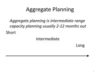
Long range Intermediate range Short range Now 2 months 1 Year Planning Horizon Aggregate planning: Intermediate-range capacity planning, usually covering 2 to 12 months.
Aggregateplanning Aggregate planning is intermediate-range capacity planning used to establish employment levels, output rates, inventory levels, subcontracting, and backorders for products that are aggregated, i.e., grouped or brought together. It does not specifically focus on individual products but deals with the products in the aggregate.
Concept of Aggregate Product For example, imagine a paint company that produces blue, brown, and pink paints; the aggregate plan in this case would be expressed as the total amount of the paint without specifying how much of it would be blue, brown or pink. Such an aggregate plan may dictate, for example, the production of 100,000 gallons of paint during an intermediate-range planning horizon, say during the whole year. The plan can later be disaggregated as to how much blue, brown, or pink paint to produce every specific time period, say every month.
Why Aggregate Planning Is Necessary • Fully load facilities and minimize overloading and underloading • Make sure enough capacity available to satisfy expected demand • Plan for the orderly and systematic change of production capacity to meet the peaks and valleys of expected customer demand • Get the most output for the amount of resources available
Aggregate Planning Strategies • Should inventoriesbe used to absorb changes in demand during planning period? • Should demand changes be accommodated by varying the size of the workforce? • Should part-timers be used, or should overtime and/or machine idle time be used to absorb fluctuations? • Should subcontractorsbe used on fluctuating orders so a stable workforce can be maintained? • Should prices or other factors be changed to influence demand?
Introduction to Aggregate Planning • Goal: To plan gross work force levels and set firm-wide production plans so that predicted demand for aggregated unitscan be met. Concept is predicated on the idea of an “aggregate unit” of production. May be actual units, or may be measured in weight (tons of steel), volume (gallons of gasoline), time (worker-hours), or dollars of sales. Can even be a fictitious quantity. (Refer to example in handout and in slide below.)
AggregationMethodSuggestedbyHaxand Meal • Hax and Meal suggest grouping products into three categories: 1. items, 2. families, and 3. types. • Items are the finest level in the product structure and correspond to individual Stock-KeepingUnits (SKU). For example, a firm selling refrigerators would distinguish whitefrom almond in the same refrigeratoras different items. • A family in this context would be refrigerators in general. • Types are natural groupings of families; kitchen appliances might be one type.
Aggregate Units The method is based on notion of aggregate units. They may be • Actual units of production • Weight (tons of steel) • Dollars (Value of sales) • Fictitious aggregate units(See example 3.1)
Example of fictitious aggregate units.(Example 3.1) One plant produced 6 models of washing machines: Model # hrs. Price % sales A 5532 4.2 285 32 K 4242 4.9 345 21 L 9898 5.1 395 17 L 3800 5.2 425 14 M 2624 5.4 525 10 M 3880 5.8 725 06 Question: How do we define an aggregate unit here?
Example continued • Notice: Price is not necessarily proportional to worker hours (i.e., cost): why? One method for defining an aggregate unit: requires: .32(4.2) + .21(4.9) + . . . + .06(5.8) = 4.8644 worker hours. This approach for this example is reasonable since products produced are similar. When products produced are heterogeneous, a natural aggregate unit is sales dollars.
Aggregate Planning • Aggregateplanningmightalso be calledmacroproductionplanning. • Whether a companyprovides a service orproduct, macroplanningbeginswiththeforecast of demand. • Aggregateplanningmethodology is designedtotranslatedemandforecastsinto a blueprintforplanning : - staffingand - productionlevels forthefirmover a predeterminedplanninghorizon.
Aggregate Planning • The aggregate planning methodology discussed in this chapter assumes that the demand is deterministicanddynamic. • This assumption is made to simplify the analysis and allow us to focus on the systematic and predictable changes in the demand pattern. • Aggregate planning involves competing objectives: - react quickly to anticipated changes in demand - retain a stable workforce - develop a production plan that maximizes profitover the planning horizon subject to constraints on capacity
Nature of Demand • Demand I. Deterministic • Static • Dynamic II. Probabilistic • Stationary • Non-Stationary • Inaggregateproductionplanning, weassumethatdemand is deterministicanddynamic.
Costs in Aggregate Planning • Smoothing Costs • changing size of the work force • changing number of units produced • Holding Costs • primary component: opportunity cost of investment in inventory • Shortage Costs • Cost of demand exceeding stock on hand. • Other Costs: payroll, overtime, idle cost, subcontracting.
Fig. 3-2 Cost of Changing the Size of the Workforce
$ Cost Slope = Ci Slope = CP Back-orders Positive inventory Inventory Fig. 3-3 Holding and Back-Order Costs
Overview of the Aggregate Production Problem Suppose that D1, D2, . . . , DT are the forecasts of demand for aggregate units over the planning horizon (T periods.) The problem is to determine both work force levels (Wt) and production levels (Pt ) to minimize total costs over the T period planning horizon.
Prototype Aggregate Planning Example(this example is not in the handout) The washing machine plant is interested in determining work force and production levels for the next 8 months. Forecasted demands for Jan-Aug. are: 420, 280, 460, 190, 310, 145, 110, 125. Starting inventory at the end of December is 200 and the company would like to have 100 units on hand at the end of August. Find monthly production levels.
Step 1: Determine “net” demand.(subtract starting inventory from period 1 forecast and add ending inventory to period 8 forecast.) Month Net Predicted Cum. Net Demand Demand 1(Jan) 220(420-200)220 2(Feb) 280 500 3(Mar) 460 960 4(Apr) 190 1150 5(May) 310 1460 6(June) 145 1605 7(July) 110 1715 8(Aug) 225(125+100) 1940
Step 2. Graph Cumulative Net Demand to Find Plans Graphically
Basic Strategies • Constant Workforce (Level Capacity)strategy: • Maintaining a steady rate of regular-time output while meeting variations in demand by a combination of options. • Zero Inventory(MatchingDemand, Chase) strategy: • Matching capacity to demand; the planned output for a period is set at the expected demand for that period.
Advantages and Disadvantages • Chase Strategy • Reduced inventory costs. • High levels of worker utilization. • Cost of fluctuating workforce levels. • Potential damage to employee morale. • Level Strategy • Worker levels and production output are stable. • High inventory costs. • Increased labor costs.
Constant Work Force Plan Suppose that we are interested in determining a production plan that doesn’t change the size of the workforce over the planning horizon. How would we do that? One method: In previous picture, draw a straight line from origin to 1940 units in month 8: The slope of the line is the number of units to produce each month.
Monthly Production = 1940/8 = 242.2 or rounded to 243/month. But: there are stockouts.
How can we have a constant work force plan with no stockouts? Answer: using the graph, find the straight line that goes through the origin and lies completely above the cumulative net demand curve:
From the previous graph, we see that cum. net demand curve is crossed at period 3, so that monthly production is 960/3 = 320. Ending inventory each month is found from: Month Cum. Net. Dem. Cum. Prod. Invent. 1(Jan) 220 320 100 2(Feb) 500 640 140 3(Mar) 960 960 0 4(Apr.) 1150 1280 130 5(May) 1460 1600 140 6(June) 1605 1920 315 7(July) 1715 2240 525 8(Aug) 1940 2560 620
But - may not be realistic for several reasons: • Since all months do not have the same number of workdays, a constant production level may not translate to the same number of workers each month.
To Overcome These Shortcomings: • Assume number of workdays per month is given (reasonable!) • Compute a “K factor” given by: K = number of aggregate units produced by one worker in one day
Finding K • Supposewe are told that over a period of 40 days, 520 units were produced with 38 workers. It follows that: • K= 520/(38*40) = .3421 average number of units produced by one worker in one day.
Computing Constant Work Force -- Realistically • Assume we are given the following # of working days per month: 22, 16, 23, 20, 21, 22, 21, 22. • March is still the critical month. • Cum. net demand thru March = 960. • Cum # working days = 22+16+23 = 61. • We find that: • 960/61 = 15.7377 units/day • 15.7377/.3421 = 46 workers required • Actually 46.003 – here we truncate because we are set to build inventory so the low number should work (check for March stock out) – however we must use care and typically ‘round up’ any fractional worker calculations thus building more inventory
Why again did we pick on March? • Examining the graph we see that March was the “Trigger point” where our constant production line intersected the cumulative demand line assuring NO STOCKOUTS! • Can we “prove” this is thebest?
Tabulate Days/Production Per Worker Versus Demand To Find Minimum Numbers
What Should We Look At? • Cumulative Demand says March needs most workers – this can be interpretted as building inventories in Jan + Feb to fulfill the greater March demand • However, if we keep this number of workers we will continue to build inventory through the rest of the plan!
Constant Work Force Production Plan Mo # wk days Prod. Cum Cum Nt End Inv Level Prod Dem Jan 22 346 346 220 126 Feb 16 252 598 500 98 Mar 23 362 960 960 0 Apr 20 315 1275 1150 125 May 21 330 1605 1460 145 Jun 22 346 1951 1605 346 Jul 21 330 2281 1715 566 Aug 22 346 2627 1940 687
Addition of Costs • Holding Cost (per unit per month): $8.50 • Hiring Cost per worker: $800 • Firing Cost per worker: $1,250 • Payroll Cost: $75/worker/day • Shortage Cost: $50 unit short/month
Cost Evaluation of Constant Work Force Plan • Assume that the work force at the end of Dec. was 40. • Cost to hire 6 workers: 6*800 = $4800 • Inventory Cost: accumulate ending inventory: (126+98+0+. . .+687) = 2093. Add in 100 units netted out in Aug = 2193. • Hence Inv. Cost = 2193*8.5=$18,640.50 • Payroll cost: ($75/worker/day)(46 workers )(167days) = $576,150 • Cost of plan: $576,150 + $18,640.50 + $4800 = $599,590.50
Cost Reduction in Constant Work Force Plan(Mixed Strategy) In the original cum net demand curve, consider making reductions in the work force one or more times over the planning horizon to decrease inventory investment.
Zero Inventory Plan (Chase Strategy) • Here the idea is to change the workforce each month in order to reduce ending inventory to nearly zero by matching the workforce with monthly demand as closely as possible. This is accomplished by computing the # of units produced by one worker each month (by multiplying K by #days per month) and then taking net demand each month and dividing by this quantity. The resulting ratio is rounded up to avoid shortages.
An Alternative is called the “Chase Plan” • Here, we hire and fire (layoff) workers to keep inventory low! • We would employ only the number of workers needed each month to meet the demand • Examining our chart (earlier) we need: • Jan: 30; Feb: 51; Mar: 59; Apr: 27; May: 43 Jun: 20; Jul: 15; Aug: 30 • Found by: (monthly demand) (monthly production/worker), for Jan= 220/(22*.3425)
An Alternative is called the “Chase Plan” • So we hire or Fire (lay-off) monthly • Jan (starts with 40 workers): Fire 10 (cost $8000) • Feb: Hire 21 (cost $16800) • Mar: Hire 8 (cost $6400) • Apr: Fire 31 (cost $38750) • May: Hire 15 (cost $12000) • Jun: Fire 23 (cost $28750) • Jul: Fire 5 (cost $6250) • Aug: Hire 15 (cost $12000) • Total Personnel Costs: $128950
Changing the Level of Work Force • Period # hired #fired • 1 10 • 2 21 • 3 8 • 4 31 • 5 15 • 6 23 • 7 5 • 8 15
An Alternative is called the “Chase Plan” • Inventory cost is essentially 165*8.5 = $1402.50 • Employment costs: $428325 • Chase Plan Total: $558677.50 • It is betterthanthe “Constant Workforce Plan” by: • 599590.50 – 558677.50 = 40913 • But will this be good for your image? • Can we find a better plan?
Example Demand for Quantum Corporation’s action toy series follows a seasonal pattern – growing through the fall months and culminating in December, with smaller peaks in January (for after-season markdowns, exchanges, and accessory purchases) and July (for Christmas-in-July specials). Each worker can produce on average 100 cases of action toys each month. Overtime is limited to 300 cases, and subcontracting is unlimited. No action toys are currently in inventory. The wage rate is $10 per case for regular production, $15 for overtime production, and $25 for subcontracting. No stockouts are allowed. Holding cost is $1 per case per month. Increasing the workforce costs approximately $1,000 per worker. Decreasing the workforce costs $500 per worker.
Example – Level Production Input:Beg. Wkrs 10 Regular $10 Hiring $1,000 Units/Wkr 100 Overtime $15 Firing $500 Cost: $146,000 Beg. Inv. 0 Subk $25 Inventory $1
Example – Chase Demand Input:Beg. Wkrs 10 Regular $10 Hiring $1,000 Units/Wkr 100 Overtime $15 Firing $500 Cost: $149,000 Beg. Inv. 0 Subk $25 Inventory $1
Disaggregating The Aggregate Plan • Disaggregation of aggregateplansmeanconverting an aggregate plan to a detailed master production schedule for each individual item (rememberthehierarchicalproductstructuregivenearlier: items, families, types). • Keep in mindthat unless the results of the aggregate plan can be linked to the master production schedule, the aggregate planning methodology could have little value.
AggregatePlanning Disaggregation MasterSchedule Aggregate Plan to Master Schedule