Download
1 / 31
400 likes | 938 Views
Aggregate Planning. Chapter 13. Beni Asllani University of Tennessee at Chattanooga. Operations Management - 5 th Edition. Roberta Russell & Bernard W. Taylor, III. Lecture Outline. Aggregate Planning Process Strategies for Adjusting Capacity Strategies for Managing Demand

E N D
Aggregate Planning Chapter 13 Beni AsllaniUniversity of Tennessee at Chattanooga Operations Management - 5th Edition Roberta Russell & Bernard W. Taylor, III Copyright 2006 John Wiley & Sons, Inc.
Lecture Outline • Aggregate Planning Process • Strategies for Adjusting Capacity • Strategies for Managing Demand • Quantitative Techniques for Aggregate Production Planning • Hierarchical Nature of Planning • Aggregate Planning for Services Copyright 2006 John Wiley & Sons, Inc.
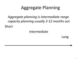
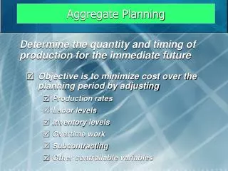
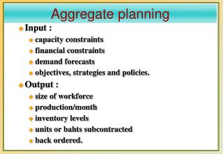
Aggregate Planning • Determine the resource capacity needed to meet demand over an intermediate time horizon • Aggregate refers to product lines or families • Aggregate planning matches supply and demand • Objectives • Establish a company wide game plan for allocating resources • Develop an economic strategy for meeting demand Copyright 2006 John Wiley & Sons, Inc.
Aggregate Planning Process Copyright 2006 John Wiley & Sons, Inc.
Meeting Demand Strategies • Adjusting capacity • Resources necessary to meet demand are acquired and maintained over the time horizon of the plan • Minor variations in demand are handled with overtime or under-time • Managing demand • Proactive demand management Copyright 2006 John Wiley & Sons, Inc.
Level production Producing at a constant rate and using inventory to absorb fluctuations in demand Chase demand Hiring and firing workers to match demand Peak demand Maintaining resources for high-demand levels Overtime and under-time Increasing or decreasing working hours Subcontracting Let outside companies complete the work Part-time workers Hiring part time workers to complete the work Backordering Providing the service or product at a later time period Strategies for Adjusting Capacity Copyright 2006 John Wiley & Sons, Inc.
Demand Production Units Time Level Production Copyright 2006 John Wiley & Sons, Inc.
Demand Production Units Time Chase Demand Copyright 2006 John Wiley & Sons, Inc.
Strategies for Managing Demand • Shifting demand into other time periods • Incentives • Sales promotions • Advertising campaigns • Offering products or services with counter-cyclical demand patterns • Partnering with suppliers to reduce information distortion along the supply chain Copyright 2006 John Wiley & Sons, Inc.
Quantitative Techniques For APP • Pure Strategies • Mixed Strategies • Linear Programming • Transportation Method • Other Quantitative Techniques Copyright 2006 John Wiley & Sons, Inc.
QUARTER SALES FORECAST (LB) Spring 80,000 Summer 50,000 Fall 120,000 Winter 150,000 Pure Strategies Example: Hiring cost = $100 per worker Firing cost = $500 per worker Regular production cost per pound = $2.00 Inventory carrying cost = $0.50 pound per quarter Production per employee = 1,000 pounds per quarter Beginning work force = 100 workers Copyright 2006 John Wiley & Sons, Inc.
Level production = 100,000 pounds SALES PRODUCTION QUARTER FORECAST PLAN INVENTORY Spring 80,000 100,000 20,000 Summer 50,000 100,000 70,000 Fall 120,000 100,000 50,000 Winter 150,000 100,000 0 400,000 140,000 Cost of Level Production Strategy (400,000 X $2.00) + (140,00 X $.50) = $870,000 (50,000 + 120,000 + 150,000 + 80,000) 4 Level Production Strategy Copyright 2006 John Wiley & Sons, Inc.
Chase Demand Strategy SALES PRODUCTION WORKERS WORKERS WORKERS QUARTER FORECAST PLAN NEEDED HIRED FIRED Spring 80,000 80,000 80 0 20 Summer 50,000 50,000 50 0 30 Fall 120,000 120,000 120 70 0 Winter 150,000 150,000 150 30 0 100 50 Cost of Chase Demand Strategy (400,000 X $2.00) + (100 x $100) + (50 x $500) = $835,000 Copyright 2006 John Wiley & Sons, Inc.
Mixed Strategy • Combination of Level Production and Chase Demand strategies • Examples of management policies • no more than x% of the workforce can be laid off in one quarter • inventory levels cannot exceed x dollars • Many industries may simply shut down manufacturing during the low demand season and schedule employee vacations during that time Copyright 2006 John Wiley & Sons, Inc.
General Linear Programming (LP) Model • LP gives an optimal solution, but demand and costs must be linear • Let • Wt = workforce size for period t • Pt =units produced in period t • It =units in inventory at the end of period t • Ft =number of workers fired for period t • Ht = number of workers hired for period t Copyright 2006 John Wiley & Sons, Inc.
LP MODEL Minimize Z = $100 (H1 + H2 + H3 + H4) + $500 (F1 + F2 + F3 + F4) + $0.50 (I1 + I2 + I3 + I4) Subject to P1 - I1 = 80,000 (1) Demand I1 + P2 - I2 = 50,000 (2) constraints I2 + P3 - I3 = 120,000 (3) I3 + P4 - I4 = 150,000 (4) Production 1000 W1 = P1 (5) constraints 1000 W2 = P2 (6) 1000 W3 = P3 (7) 1000 W4 = P4 (8) 100 + H1 - F1 = W1 (9) Work force W1 + H2 - F2 = W2 (10) constraints W2 + H3 - F3 = W3 (11) W3 + H4 - F4 = W4 (12) Copyright 2006 John Wiley & Sons, Inc.
EXPECTED REGULAR OVERTIME SUBCONTRACT QUARTER DEMAND CAPACITY CAPACITY CAPACITY 1 900 1000 100 500 2 1500 1200 150 500 3 1600 1300 200 500 4 3000 1300 200 500 Regular production cost per unit $20 Overtime production cost per unit $25 Subcontracting cost per unit $28 Inventory holding cost per unit per period $3 Beginning inventory 300 units Transportation Method Copyright 2006 John Wiley & Sons, Inc.
PERIOD OF USE Unused PERIOD OF PRODUCTION 1 2 3 4 Capacity Capacity 1 2 3 4 Beginning 0 3 6 9 Inventory 300 — — — 300 Regular 600 300 100 — 1000 Overtime 100 100 Subcontract 500 Regular 1200 — — 1200 Overtime 150 150 Subcontract 250 250 500 Regular 1300 — 1300 Overtime 200 — 200 Subcontract 500 500 Regular 1300 1300 Overtime 200 200 Subcontract 500 500 Demand 900 1500 1600 3000 250 20 23 26 29 25 28 31 34 28 31 34 37 20 23 26 25 28 31 28 31 34 20 23 25 28 28 31 20 25 28 Transportation Tableau
REGULAR SUB- ENDING PERIOD DEMAND PRODUCTION OVERTIME CONTRACT INVENTORY 1 900 1000 100 0 500 2 1500 1200 150 250 600 3 1600 1300 200 500 1000 4 3000 1300 200 500 0 Total 7000 4800 650 1250 2100 Burruss’ Production Plan Copyright 2006 John Wiley & Sons, Inc.
Other Quantitative Techniques • Linear decision rule (LDR) • Search decision rule (SDR) • Management coefficients model Copyright 2006 John Wiley & Sons, Inc.
Production Planning Capacity Planning Resource Level Items Aggregate production plan Resource requirements plan Product lines or families Plants Master production schedule Rough-cut capacity plan Critical work centers Individual products Material requirements plan Capacity requirements plan All work centers Components Shop floor schedule Input/ output control Manufacturing operations Individual machines Hierarchical Nature of Planning Copyright 2006 John Wiley & Sons, Inc.
Available-to-Promise (ATP) • Quantity of items that can be promised to the customer • Difference between planned production and customer orders already received AT in period 1 = (On-hand quantity + MPS in period 1) – - (CO until the next period of planned production) ATP in period n = (MPS in period n) – - (CO until the next period of planned production) Copyright 2006 John Wiley & Sons, Inc.
ATP: Example Copyright 2006 John Wiley & Sons, Inc.
ATP: Example (cont.) Copyright 2006 John Wiley & Sons, Inc.
= 30 = 0 ATP: Example (cont.) Take excess units from April ATP in April = (10+100) – 70 = 40 ATP in May = 100 – 110 = -10 ATP in June = 100 – 50 = 50 Copyright 2006 John Wiley & Sons, Inc.
Product Request Is an alternative product available at an alternate location? Yes Yes Is the product available at this location? Available-to-promise No No Allocate inventory Capable-to-promise date Yes Is an alternative product available at this location? Available-to-promise Is the customer willing to wait for the product? No Yes Allocate inventory Revise master schedule Is this product available at a different location? Yes No Trigger production Lose sale No Rule Based ATP Copyright 2006 John Wiley & Sons, Inc.
Aggregate Planning for Services Most services can’t be inventoried Demand for services is difficult to predict Capacity is also difficult to predict Service capacity must be provided at the appropriate place and time Labor is usually the most constraining resource for services Copyright 2006 John Wiley & Sons, Inc.
Yield Management Copyright 2006 John Wiley & Sons, Inc.
Yield Management (cont.) Copyright 2006 John Wiley & Sons, Inc.
NO-SHOWS PROBABILITY P(N < X) 0 .15 .00 1 .25 .15 2 .30 .40 3 .30 .70 .517 Optimal probability of no-shows P(n < x) = = .517 Cu Cu + Co 75 75 + 70 Yield Management: Example Hotel should be overbooked by two rooms Copyright 2006 John Wiley & Sons, Inc.
Copyright 2006 John Wiley & Sons, Inc.All rights reserved. Reproduction or translation of this work beyond that permitted in section 117 of the 1976 United States Copyright Act without express permission of the copyright owner is unlawful. Request for further information should be addressed to the Permission Department, John Wiley & Sons, Inc. The purchaser may make back-up copies for his/her own use only and not for distribution or resale. The Publisher assumes no responsibility for errors, omissions, or damages caused by the use of these programs or from the use of the information herein. Copyright 2006 John Wiley & Sons, Inc.