Download
1 / 59
590 likes | 595 Views
This lecture outlines the basics of computer graphics, the types of data we will study (fields and meshes), and the concept of interpolation. It also covers the goals and due dates for Project #1 and #2. The lecture distinguishes between scientific visualization and information visualization, and discusses the use of visualization for communication, confirmation, and exploration. Additionally, it explains the basics of using a graphics system and the elements of a visualization. Lastly, it addresses potential errors and ways that visualization can lie.

E N D
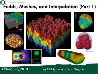
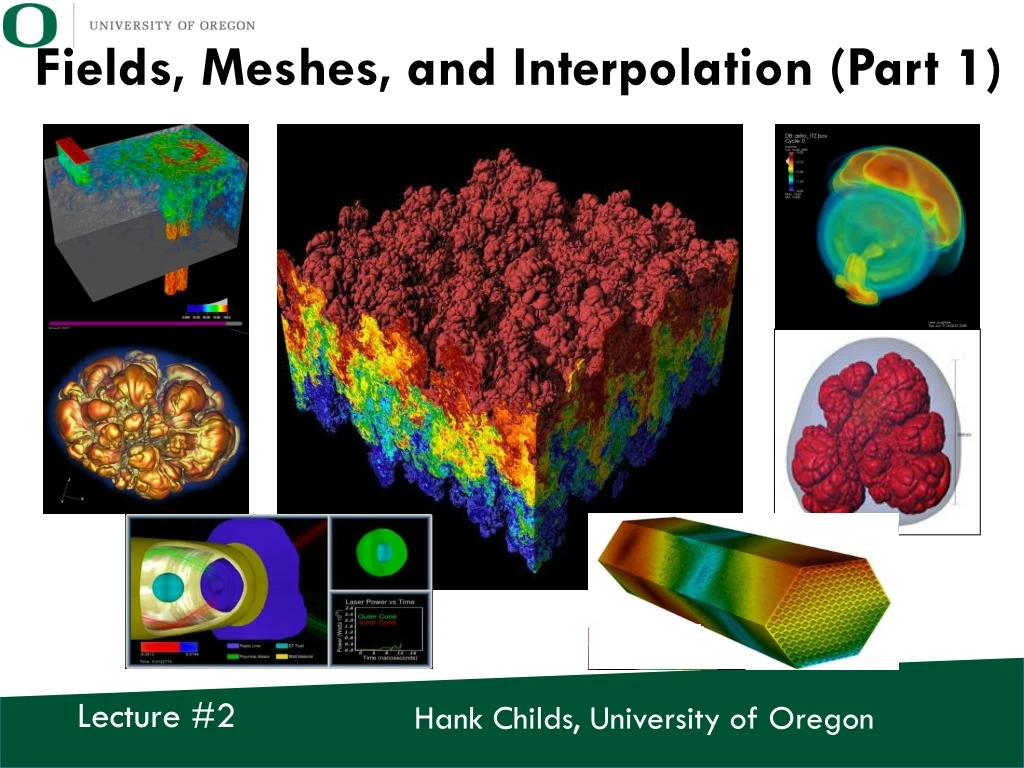
Fields, Meshes, and Interpolation (Part1) Hank Childs, University of Oregon Lecture #2
Outline • Projects & OH • Intro • SciVisvsInfoVis • Very, very basics of computer graphics • The Data We Will Study • Overview • Fields • Meshes • Interpolation
Outline • Projects & OH • Intro • SciVisvsInfoVis • Very, very basics of computer graphics • The Data We Will Study • Overview • Fields • Meshes • Interpolation
Project #1: how’s it going? Goal: write a specific image Due: “Friday Jan 12th” “6am Saturday Jan 13th” % of grade: 2% Goal: get multi-platform issues shaken out ASAP. Experience last year was pretty good.
Project #2 • Will assign on Friday • Don’t want to have to rush through lecture … will only make things confusing.
Office Hours • Hank: • Tuesday 11-12 • Thursday 1-230 • Brent • Monday 3-4 • Wednesday 3-4 • (is this ok?) • Also: Brent available this week by appointment
Outline • Projects & OH • Intro • SciVisvsInfoVis • Very, very basics of computer graphics • The Data We Will Study • Fields • Meshes • Interpolation
Scientific Visualization • An interdisciplinary branch of science • primarily concerned with the visualization of three-dimensional phenomena (architectural, meteorological, medical, biological, etc.) • the emphasis is on realistic renderings of volumes, surfaces, illumination sources, and so forth, perhaps with a dynamic (time) component. • It is also considered a branch of computer science that is a subset of computer graphics. • The purpose of scientific visualization is to graphically illustrate scientific data to enable scientists to understand, illustrate, and glean insight from their data. Source: wikipedia
Information Visualization • The study of (interactive) visual representations of abstract data to reinforce human cognition. • The abstract data include both numerical and non-numerical data, such as text and geographic information. Source: wikipedia
Kaela’s question • Think of data as records • One piece of data: • (x1, x2, x3, x4) • Example 1: • x1 = my age, x2 = my height, x3 = my weight, x4 = my vertical leap • Example 2: • x1 = latitude position, x2 = longitude position, x3 = elevation, x4 = temperature at location (x1,x2,x3) • If each data record has a location *and* if you want to visualize using that location, then it is scientific visualization.
SciVisvsInfoVis • “it’s infoviswhen the spatial representation is chosen, and it’s scivis when the spatial representation is given” (A) (C) (B) (D) (E)
What sorts of data? Of course, lots of other data too…
What Is Visualization Used For? • 3 Main Use Cases: • Communication • Confirmation • Exploration
How Visualization Works • Many visual metaphors for representing data • How to choose the right tool from the toolbox? • This course: • Describe the tools • Describe the systems that support the tools
Outline • Projects & OH • Intro • SciVisvsInfoVis • Very, very basics of computer graphics • The Data We Will Study • Overview • Fields • Meshes • Interpolation
Computer Graphics Defined: pictorial computer output produced, through the use of software, on a display screen, plotter, or printer.
What is computer graphics good for? • Ed Angel book: • Display of information • Design • Simulation and animation • User interfaces
The Basics of Using a Graphics System • You define: • Geometric primitives, typically a triangle mesh • Coloring for those geometry primitives • A model for a camera (where you are and what you are looking at) • And then: • Communicate this information using an interface (e.g., OpenGL) • And something (e.g., GPU) renders the scene • VTK will do this for us. • Visualization: We will focus on transforming data to geometric primitives.
Outline • Projects & OH • Intro • SciVisvsInfoVis • Very, very basics of computer graphics • The Data We Will Study • Overview • Fields • Meshes • Interpolation
Elements of a Visualization Legend Provenance Information Reference Cues Display of Data
Elements of a Visualization What is the value at this location? How do you know? What data went into making this picture?
Where does temperature data come from? • Iowa circa 1980s: people phoned in updates What is the temperature along the white line? 6:00pm: Grandma’s friend calls in 82F. 6:00pm: Grandma calls in 80F.
What is the temperature at points between Ralston and Glidden? 82F Temperature 81F 80F ~ ~ D=0, Ralston, IA D=10 miles, Glidden, IA Distance
Ways Visualization Can Lie Visualization Errors: Illusion of certainty Poor choices of parameters Visualization Program Data Errors: Data collection is inaccurate Data collected too sparsely
Outline • Projects & OH • Intro • SciVisvsInfoVis • Very, very basics of computer graphics • The Data We Will Study • Overview • Fields • Meshes • Interpolation
Fields & Spaces • Fields are defined over “spaces”. • We will be considering 2D & 3D spaces. • Defined by an origin and three vectors (or two vectors) that define orientation.
Scalar Fields The temperature at 41.2324° N, 98.4160° W is 66F. • Defined: associate a scalar with every point in space. • What is a scalar? • A: a real number • Examples: • Temperature • Density • Pressure Fields are defined at every location in a space (example space: USA)
Vector Fields The velocity at location (5, 6) is (-0.1, -1) The velocity at location (10, 5) is (-0.2, 1.5) • Defined: associate a vector with every point in space. • What is a vector? • A: a direction and a magnitude • Examples: • Velocity Typically, 2D spaces have 2 components in their vector field, and 3D spaces have 3 components in their vector field.
Vector Fields Representing dense vector data is hard and requires special techniques.
More fields (discussed later in course) • Tensor fields • Functions • Volume fractions • Multi-variate data
Outline • Projects & OH • Intro • SciVisvsInfoVis • Very, very basics of computer graphics • The Data We Will Study • Overview • Fields • Meshes • Interpolation
Mesh What we want
An example mesh Where is the data on this mesh? (for today, it is at the vertices of the triangles)
An example mesh Why do you think the triangles change size?
Anatomy of a computational mesh • Meshes contain: • Cells • Points • This mesh contains 3 cells and 13 vertices • Pseudonyms: • Cell == Element == Zone • Point == Vertex == Node
Types of Meshes Adaptive Mesh Refinement Curvilinear Unstructured We will discuss all of these mesh types more later in the course.
Rectilinear meshes • Rectilinear meshes are easy and compact to specify: • Locations of X positions • Locations of Y positions • 3D: locations of Z positions • Then: mesh vertices are at the cross product. • Example: • X={0,1,2,3} • Y={2,3,5,6} Y=6 Y=5 Y=3 Y=2 X=0 X=1 X=2 X=3
Rectilinear meshes aren’t just the easiest to deal with … they are also very common
Quiz Time • A 3D rectilinear mesh has: • X = {1, 3, 5, 7, 9} • Y = {2, 3, 5, 7, 11, 13, 17} • Z = {1, 2, 3, 5, 8, 13, 21, 34, 55} • How many points? • How many cells? = 5*7*9 = 315 Y=6 = 4*6*8 = 192 Y=5 Y=3 Y=2 X=0 X=1 X=2 X=3
Definition: dimensions • A 3D rectilinear mesh has: • X = {1, 3, 5, 7, 9} • Y = {2, 3, 5, 7, 11, 13, 17} • Z = {1, 2, 3, 5, 8, 13, 21, 34, 55} • Then its dimensions are 5x7x9
How to Index Points • Motivation: many algorithms need to iterate over points. for (inti = 0 ; i < numPoints ;i++) { double *pt = GetPoint(i); AnalyzePoint(pt); }
Schemes for indexing points Point indices Logical point indices What would these indices be good for?
How to Index Points • Problem description: define a bijective function, F, between two sets: • Set 1: {(i,j,k): 0<=i<nX, 0<=j<nY, 0<=k<nZ} • Set 2: {0, 1, …, nPoints-1} • Set 1 is called “logical indices” • Set 2 is called “point indices” Bijective: for every element in set 1, there is an element in set 2. And vice-versa. Note: for the rest of this presentation, we will focus on 2D rectilinear meshes.
How to Index Points • Many possible conventions for indexing points and cells. • Most common variants: • X-axis varies most quickly • X-axis varies most slowly F
Bijective function for rectilinear meshes for this course intGetPoint(inti, int j, intnX, intnY) { return j*nX + i; } F
Bijective function for rectilinear meshes for this course int *GetLogicalPointIndex(int point, intnX, intnY) { intrv[2]; rv[0] = point % nX; rv[1] = (point/nX); return rv; // terrible code!! }
int *GetLogicalPointIndex(int point, intnX, intnY) { intrv[2]; rv[0] = point % nX; rv[1] = (point/nX); return rv; } F
Quiz Time #2 • A mesh has dimensions 6x8. • What is the point index for (3,7)? • What are the logical indices for point 37? = 45 = (1,6) int *GetLogicalPointIndex(int point, intnX, intnY) { intrv[2]; rv[0] = point % nX; rv[1] = (point/nX); return rv; // terrible code!! } intGetPoint(inti, int j, intnX, intnY) { return j*nX + i; }