Download
1 / 16
160 likes | 263 Views
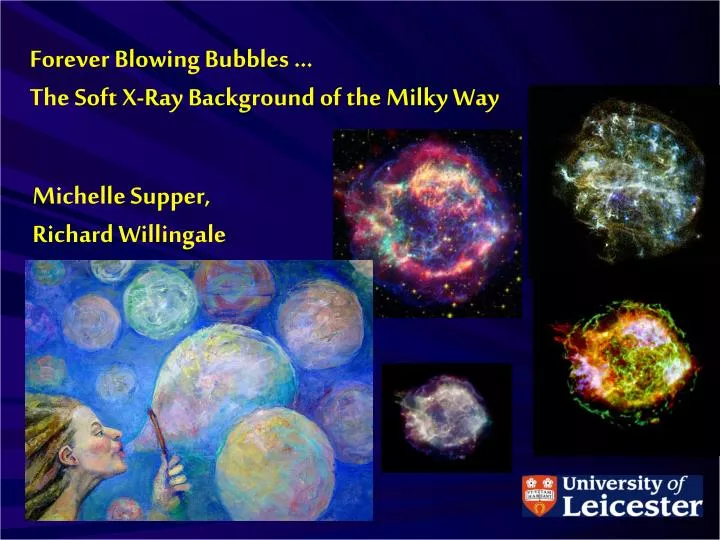
Forever Blowing Bubbles … The Soft X-Ray Background of the Milky Way. Michelle Supper, Richard Willingale. Overview. Why look at it? The observations How to extract the spectra Modelling Results Ideas and Interpretations. Why look at the SXRB?.

E N D
Forever Blowing Bubbles … The Soft X-Ray Background of the Milky Way Michelle Supper, Richard Willingale
Overview • Why look at it? • The observations • How to extract the spectra • Modelling • Results • Ideas and Interpretations
Why look at the SXRB? • Uncertain: Chemical composition, origin, heating mechanism, morphology. • Featureless: Except at soft photon energies 0.1–4.0 keV • Structures: Visible inROSAT All-Sky Survey (RASS)
The RASS ¾ KeV Map Loop 1 North Polar Spur Galactic Plane
Observations: Within Loop 1 • 3 fields in the North • 5 fields in the South • 2 fields in the North Polar Spur • Allows variations to be measured as a function of latitude NPS X3 X2 X1 B1 B2 B3 B4 B5
Unusual Steps in Data Reduction: • Light curve heavily filtered to remove flares and hot pixels. • Mask out point sources • Cosmic ray contamination estimated from unexposed chip corners.
Reduced EPIC Spectra: PN Data 1 MOS Data 0.1 Normalised Counts/sec/keV 0.01 Al K and Si K from EPIC 10-3 0.5 1.0 2.0 Channel Energy (keV)
LHB (Northern fields projection) NPS fields Northern Bulge Fields Cold Column Loop1 Superbubble Galactic Bulge The Wall Southern Bulge Fields LHB (Southern fields projection) Local Hot Bubble Cool Halo Loop 1 Galactic Plane Cosmic Background Earth nH nH nH nH (Apec) (Wabs x Vapec) (Wabs x Apec) (Wabs x Bknpower) (Wabs x ? ) What’s going on, and how to model it…
The Model ApecLHB: Fixed temperature 0.1keV. Dominates 0.5keV. + (WabsNPS: Temperature ~0.3keV. Dominates 0.4 - 0.75keV. x Vapec) Fits the O VIII, Fe XVII, Ne IX and Mg XI emission lines. Absorption represents the Wall. + (Wabs x Extra Component MEKAL) Temperature set at 2 KeV. Absorption frozen to galactic nH. + (Wabs xGalactic Halo: fixed temperature 0.1KeV. Apec) Dominates the 0.4-0.6 keV region. O VII line is a prominent feature. Absorption frozen to galactic nH. + (Wabs xCosmic Background Bknpower)Absorption frozen to galactic nH.
Fitted Spectrum 1 0.1 Normalised Counts/sec/keV 0.01 OVII OVIII FeXII NeIX NeX 10-3 0.2 1.0 2.0 0.5 Channel Energy (keV)
LHB (Northern fields projection) NPS fields Northern Bulge Fields Cold Column Loop1 Superbubble Galactic Bulge The Wall Southern Bulge Fields LHB (Southern fields projection) Analysis: Modelling Distances Loop 1 Centre: (325°, 25°) Distance to centre: 210 parsecs Diameter: 276 parsecs (Radius 138 parsecs)
LHB The Wall Loop1 N5 N4 Increasing density Increasing pressure Latitude = 25° X3 X2 X1 SNR Interaction? • LHB emission measure ~ constant (6 x 10⁻⁴ cm-6 pc) • LHB electron pressure: increases towards 25° latitude. • Distance to the Wall: increases sharply from X3 B5 (28 110 parsecs) • Density of the Wall: higher in N4 than N5, very high in the south (3 x higher). • INTERACTION?
The Extra Component… • Hard component, modelled as 2 keV Mekal • Required only in 6° nearest the Plane • Increases quickly near plane • Associated with Plane or Galactic Centre? • Can’t check for presence in the North North Polar Spur Fields Northern Fields Southern Fields Loop 1 model boundary
Chemical Abundances in Loop 1 • Depleted Shell • Rich, high abundances in centre
Galactic halo = MYSTERY. Count photons in range Determine flux contribution from each component Hence Trace 0.1keV plasma, try to determine its origin. Investigate the distribution of the Galactic Halo Next Steps: Oxygen in the Halo
Berkhuijsen E., Haslam C., Salter C., 1971, A&A, 14, 252-262 Egger R. J., Aschenbach B., 1995, A&A, 294, L25-L28 Snowden S. L. et al., 1995, ApJ, 454, 643-653 Snowden S. L. et al., 1997, ApJ, 485, 125-135 Willingale R., XMM AO-2 Proposal Willingale R., Hands A. D. P., Warwick R. S., Snowden S. L., Burrows D. N., 2003, MNRAS, 343, 995-1001. The End! <wake up> mar23@star.le.ac.uk References Any Questions?