Classification (Discrimination, Supervised Learning) Using Microarray Data
Classification (Discrimination, Supervised Learning) Using Microarray Data. Xuelian Wei Department of Statistics Most of Slides Adapted from http://statwww.epfl.ch/davison/teaching/Microarrays/ by Darlene Goldstein. Gene expression data. mRNA samples.

Classification (Discrimination, Supervised Learning) Using Microarray Data
E N D
Presentation Transcript
Classification (Discrimination, Supervised Learning) Using Microarray Data Xuelian Wei Department of Statistics Most of Slides Adapted from http://statwww.epfl.ch/davison/teaching/Microarrays/ by Darlene Goldstein
Gene expression data mRNA samples Normal Normal Normal Cancer Cancer sample1 sample2 sample3 sample4 sample5 … 1 0.46 0.30 0.80 1.51 0.90 ... 2 -0.10 0.49 0.24 0.06 0.46 ... 3 0.15 0.74 0.04 0.10 0.20 ... 4 -0.45 -1.03 -0.79 -0.56 -0.32 ... 5 -0.06 1.06 1.35 1.09 -1.09 ... Genes Gene expression level of gene i in mRNA samplej
Tumor Classification Using Gene Expression Data Three main types of statistical problems associated with the microarray data: • Identification of “marker” genes that characterize the different tumor classes (feature or variable selection). • Identification of new/unknown tumor classes using gene expression profiles (unsupervised learning – clustering) • Classification of sample into known classes (supervised learning – classification)
Classification Y Normal Normal Normal Cancer Cancer unknown =Y_new • Each object (e.g. arrays or columns)associated with a class label (or response) Y {1, 2, …, K} and a feature vector (vector of predictor variables) of G measurements: X = (X1, …, XG) • Aim: predict Y_new from X_new. sample1 sample2 sample3 sample4 sample5 … New sample 1 0.46 0.30 0.80 1.51 0.90 ... 0.34 2 -0.10 0.49 0.24 0.06 0.46 ... 0.43 3 0.15 0.74 0.04 0.10 0.20 ... -0.23 4 -0.45 -1.03 -0.79 -0.56 -0.32 ... -0.91 5 -0.06 1.06 1.35 1.09 -1.09 ... 1.23 X X_new
Classifiers • A predictor or classifier partitions the space of gene expression profiles into K disjoint subsets, A1, ..., AK, such that for a sample with expression profile X=(X1, ...,XG)Ak the predicted class is k. • Classifiers are built from a learning set (LS) L = (X1, Y1), ..., (Xn,Yn) • Classifier C built from a learning set L: C( . ,L): X {1,2, ... ,K} • Predicted class for observation X: C(X,L) = k if X is in Ak
Classification Methods • Fisher Linear Discriminant Analysis. • Maximum Likelihood Discriminant Rule. • Quadratic discriminant analysis (QDA). • Linear discriminant analysis (LDA, equivalent to FLDA for K=2). • Diagnal quadratic discriminant analysis (DQDA). • Diagnal linear discriminant analysis (DLDA). • Nearest Neighbor Classification. • Classification and Regression Tree (CART). • Aggregating & Bagging.
Fisher Linear Discriminant Analysis -- M.Barnard. The secular variations of skull characters in four series of egyptian skulls. Annals of Eugenics, 6:352-371, 1935. -- R.A.Fisher. The use of multiple measurements in taxonomic problems. Annals of Eugenics, 7:179-188, 1936.
Fisher Linear Discriminant Analysis • In a two-class classification problem, given n samples in a d-dimensional feature space. n1 in class 1 and n2 in class 2. • Goal: to find a vector w, and project the n samples on the axis y=w’x, so that the projected samples are well separated.
Fisher Linear Discriminant Analysis • The sample mean vector for the ith class is mi and the sample covariance matrix for the ith class is Si. • The between-class scatter matrix is: SB=(m1-m2)(m1-m2)’ • The within-class scatter matrix is: Sw= S1+S2 • The sample mean of the projected points in the ith class is: • The variance of the projected points in the ith class is:
Fisher Linear Discriminant Analysis The fisher linear discriminant analysis will choose the w, which maximize: i.e. the between-class distance should be as large as possible, meanwhile the within-class scatter should be as small as possible.
Fisher Linear Discriminant Analysis For K=2, FLDA yields the same classifier as the Lear maximum likelihood discriminant rule.
Maximum Likelihood Discriminant Rule • A maximum likelihood classifier (ML) chooses the class that makes the chance of the observations the highest • Assume the condition density for each class is • the maximum likelihood (ML) discriminant rule predicts the class of an observationX by that which gives the largest likelihood to X, i.e., by
Gaussian ML Discriminant Rules • Assume the conditional densities for each class is a multivariate Gaussian (normal), P(X|Y= k) ~ N(k,k), • Then ML discriminant rule is C(X) = argmink {(X - k) k-1(X - k)’ + log| k |} • In general, this is a quadraticrule (Quadratic discriminant analysis, or QDA in R) • In practice, population mean vectors k and covariance matrices k are estimated from learning set L.
Gaussian ML Discriminant Rules • When all class densities have the same covariance matrix, k = the discriminant rule is linear(Linear discriminant analysis,orLDA in R;FLDA for k = 2): C(X) = argmink (X - k) -1(X - k)’ • In practice, population mean vectors k and constant covariance matrices are estimated from learning set L.
Gaussian ML Discriminant Rules • When the class densities have diagonal covariance matrices, , the discriminant rule is given by additive quadratic contributions from each variable(Diagonal quadratic discriminant analysis, orDQDA) • When all class densities have the same diagonal covariance matrix =diag(12… G2), the discriminant rule is again linear(Diagonal linear discriminant analysis, orDLDA in R)
Application of ML discriminant Rule • Weighted gene voting method. (Golub et al. 1999) • One of the first application of a ML discriminant rule to gene expression data. • This methods turns out to be a minor variant of the sample Diagonal Linear Discriminant rule. • Golub TR, Slonim DK, Tamayo P, Huard C, Gaasenbeek M, Mesirov JP,Coller H, Loh ML, Downing JR, Caligiuri MA, Bloomfield CD, Lander ES. (1999).Molecular classification of cancer: class discovery and class prediction bygene expression monitoring. Science. Oct 15;286(5439):531 - 537.
Example: Weighted gene voting method • Weighted gene voting method. (Golub et al. 1999)
Example: Weighted Voting method vs Diagonal Linear discriminant rule
Nearest Neighbor Classification • Based on a measure of distance between observations (e.g. Euclidean distance or one minus correlation). • k-nearest neighbor rule (Fix and Hodges (1951)) classifies an observation X as follows: • find the k closest observations in the training data, • predict the class by majority vote, i.e. choose the class that is most common among those k neighbors. • k is a parameter, the value of which will be determined by minimizing the cross-validation error later. • E. Fix and J. Hodges. Discriminatory analysis. Nonparametric discrimination: Consistency properties. Tech. Report 4, USAF School of Aviation Medicine, Randolph Field, Texas, 1951.
CART: Classification TreeBINARY RECURSIVE PARTITIONING TREE • Binary -- split parent node into two child nodes • Recursive -- each child node can be treated as parent node • Partitioning -- data set is partitioned into mutually exclusive subsets in each split -- L.Breiman, J.H. Friedman, R. Olshen, and C.J. Stone. Classification and regression trees. The Wadsworth statistics/probability series. Wadsworth International Group, 1984.
Classification Trees • Binary tree structured classifiers are constructed by repeated splits of subsets (nodes) of the measurement space X into two descendant subsets (starting with X itself) • Each terminal subset is assigned a class label; the resulting partition of X corresponds to the classifier • RPART in R or TREE in R
Three Aspects of Tree Construction • Split Selection Rule • Split-stopping Rule • Class assignment Rule • Different tree classifiers use different approaches to deal with these three issues, e.g. CART( Classification And Regression Trees)
Three Rules (CART) • Splitting: At each node, choose split maximizing decrease in impurity (e.g.Gini index, entropy, misclassification error). • Split-stopping: Grow large tree, prune to obtain a sequence of subtrees, then use cross-validation to identify the subtree with lowest misclassification rate. • Class assignment: For each terminal node, choose the class with the majority vote.
Comparison • Iris Data • Y: 3 species, • Iris setosa (red), versicolor (green), and virginica (blue). • X: 4 variables • Sepal length and width • Petal length and width (ignored!)
Other Classifiers Include… • Support vector machines (SVMs) • Neural networks • HUNDREDS more… • The Best Reference: Google
Aggregating classifiers • Breiman (1996, 1998) found that gains in accuracy could be obtained by aggregating predictors built from perturbed versions of the learning set; the multiple versions of the predictor are aggregated by weighted voting. • Let C(., Lb) denote the classifier built from the b-th perturbed learning set Lb, and let wbdenote the weight given to predictions made by this classifier. The predicted class for an observation x is given by argmaxk ∑b wbI(C(x,Lb) = k) -- L. Breiman. Bagging predictors. Machine Learning, 24:123-140, 1996. -- L. Breiman. Out-of-bag eatimation. Technical report, Statistics Department, U.C. Berkeley, 1996. -- L. Breiman. Arcing classifiers. Annals of Statistics, 26:801-824, 1998.
Aggregating Classifiers • The key to improved accuracy is the possible instability of the prediction method, i.e., whether small changes in the learning set result in large changes in the predictor. • Unstable predictors tend to benefit the most from aggregation. • Classification trees (e.g.CART) tend to be unstable. • Nearest neighbor classifier tend to be stable.
Bagging & Boosting • Two main methods for generating perturbed versions of the learning set. • Bagging. -- L. Breiman. Bagging predictors. Machine Learning, 24:123-140, 1996. • Boosting. -- Y.Freund and R.E.Schapire. A decision-theoretic generalization of on-line learning and an application to boosting. Journal of computer and system sciences, 55:119-139, 1997.
Bagging= Bootstrap aggregatingI. Nonparametric Bootstrap (BAG) • Nonparametric Bootstrap (standard bagging). • perturbed learning sets of the same size as the original learning set are formed by randomly selecting samples with replacement from the learning sets; • Predictors are built for each perturbed dataset and aggregated by plurality voting plurality voting (wb=1), i.e., the “winning” class is the one being predicted by the largest number of predictors.
Bagging= Bootstrap aggregatingII. Parametric Bootstrap (MVN) • Parametric Bootstrap. • Perturbed learning sets are generated according to a mixture of multivariate normal (MVN) distributions. • The conditional densities for each class is a multivariate Gaussian (normal), i.e., P(X|Y= k) ~ N(k,k), the sample mean vector and sample covariance matrix will be used to estimate the population mean vector and covariance matrix. • The class mixing probabilities are taken to be the class proportions in the actual learning set. • At least one observation be sampled from each class. • Predictors are built for each perturbed dataset and aggregated by plurality voting plurality voting (wb=1).
Bagging= Bootstrap aggregatingIII. Convex pseudo-data (CPD) • Convex pseudo-data. One perturbed learning set are generated by repeating the following n times: • Select two samples (x,y) and (x’, y’) at random form the learning set L. • Select at random a number of v from the interval [0,d], 0<=d<=1, and let u=1-v. • The new sample is (x’’, y’’) where y’’=y and x’’=ux+vx’ • Note that when d=0, CPD reduces to standard bagging. • Predictors are built for each perturbed dataset and aggregated by plurality voting plurality voting (wb=1).
Boosting • The perturbed learning sets are re-sampled adaptively so that the weights in the re-sampling are increased for those cases most often misclassified. • The aggregation of predictors is done by weighted voting (wb != 1).
Boosting • Learning set: L = (X1, Y1), ..., (Xn,Yn) • Re-sampling probabilities p={p1,…, pn}, initialized to be equal. • The bth step of the boosting algorithm is: • Using the current re-sampling prob p, sample with replacement from L to get a perturbed learning set Lb. • Build a classifier C(., Lb) based on Lb. • Run the learning set L through the classifier C(., Lb) and let di=1 if the ith case is classified incorrectly and let di=0 otherwise. • Define and update the re-sampling prob for the (b+1)st step by • The weight for each classifier is
Comparison of classifiers • Dudoit, Fridlyand, Speed (JASA, 2002) • FLDA (Fisher Linear Discriminant Analysis) • DLDA (Diagonal Linear Discriminant Analysis) • DQDA (Diagonal Quantic Discriminant Analysis) • NN (Nearest Neighbour) • CART (Classification and Regression Tree) • Bagging and boosting • Bagging (Non-parametric Bootstrap ) • CPD (Convex Pseudo Data) • MVN (Parametric Bootstrap) • Boosting -- Dudoit, Fridlyand, Speed: “Comparison of discrimination methods for the classification of tumors using gene expression data”, JASA, 2002
Comparison study datasets • Leukemia – Golub et al. (1999) n = 72 samples, G = 3,571 genes 3 classes (B-cell ALL, T-cell ALL, AML) • Lymphoma – Alizadeh et al. (2000) n = 81 samples, G = 4,682 genes 3 classes (B-CLL, FL, DLBCL) • NCI 60 – Ross et al. (2000) N = 64 samples, p = 5,244 genes 8 classes
Procedure • For each run (total 150 runs): • 2/3 of sample randomly selected as learning set (LS), rest 1/3 as testing set (TS). • The top p genes with the largest BSS/WSS are selected using the learning set. • p=50 for lymphoma dataset. • p=40 for leukemia dataset. • p=30 for NCI 60 dataset. • Predictors are constructed and error rated are obtained by applying the predictors to the testing set.
Leukemia data, 2 classes: Test set error rates;150 LS/TS runs
Leukemia data, 3 classes: Test set error rates;150 LS/TS runs
Lymphoma data, 3 classes: Test set error rates; N=150 LS/TS runs
Results • In the main comparison of Dudoit et al, NN and DLDA had the smallest error rates, FLDA had the highest • For the lymphoma and leukemia datasets, increasing the number of genes to G=200 didn't greatly affect the performance of the various classifiers; there was an improvement for the NCI 60 dataset. • More careful selection of a small number of genes (10) improved the performance of FLDA dramatically
Comparison study – Discussion (I) • “Diagonal” LDA: ignoring correlation between genes helped here. Unlike classification trees and nearest neighbors, LDA is unable to take into account gene interactions • Although nearest neighbors are simple and intuitive classifiers, their main limitation is that they give very little insight into mechanisms underlying the class distinctions
Comparison study – Discussion (II) • Variable selection: A crude criterion such as BSS/WSS may not identify the genes that discriminate between all the classes and may not reveal interactions between genes • With larger training sets, expect improvement in performance of aggregated classifiers
Acknowledgements • Some of slides adapted form http://statwww.epfl.ch/davison/teaching/Microarrays/ by Darlene Goldstein Thank you!