Download
1 / 35
350 likes | 548 Views
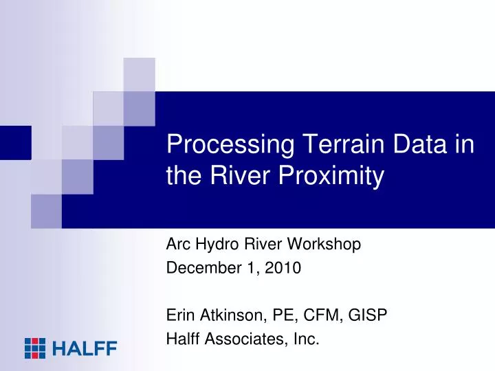
Processing Terrain Data in the River Proximity. Arc Hydro River Workshop December 1, 2010 Erin Atkinson, PE, CFM, GISP Halff Associates, Inc. Terrain Processing Overview. Terrain Data Models Terrain for Hydraulics (GeoRAS) Terrain Acquisition and LIDAR ESRI Terrain Dataset

E N D
Processing Terrain Data in the River Proximity Arc Hydro River Workshop December 1, 2010 Erin Atkinson, PE, CFM, GISP Halff Associates, Inc.
Terrain Processing Overview • Terrain Data Models • Terrain for Hydraulics (GeoRAS) • Terrain Acquisition and LIDAR • ESRI Terrain Dataset • Hydraulics and LIDAR Case Studies
Terrain for H&H Modeling • Terrain is the most important piece of data for automated H&H • Always start with source data (when possible) • Mass points • Breaklines • Contours and DEMs are typically derivative datasets • Don’t overlap data from different sources
Supported Terrain Data Models in GIS • Vector – Points, Breaklines, & Contours • Vector features representing elevation with x,y,z coordinates • DEM – Digital Elevation Model • Raster features representing terrain with cells • TIN – Triangulated Irregular Network • Nodes and edges forming triangles • ESRI Terrain Dataset
Terrain for Hydraulics • Geoprocessing tools for hydraulics usually work with TINs, but rasters are also supported • TINs allow for more detail in channel area, less in overbanks • TINs for hydraulics should be limited to the floodplain • A TIN for an entire subbasin is a waste of space and processing • Cross sections and other hydraulic features get elevation values at: • Intersection of triangle edge in a TIN • Crossing a cell in a raster
GeoRAS Elevation Dataset Requirements • GeoRAS currently supports two DTM types • TINs • GRIDs • DTM should cover channel and overbank areas • i.e. Spatial extent of DTM must cover cross sections • Terrain datasets are currently not supported by GeoRAS • GeoRAS does support the use of multiple DTMs for modeling long reaches
GeoRAS Elevation Dataset • TINs are recommended for use with GeoRAS • Linear features can be enforced • Channel banks • Hydraulic structures • Roads • Density of data can be varied (channel vs. overbank) • Survey information can be retained
Terrain Acquisition Methods • Remote sensing technologies are collecting data at very fine resolutions • LIDAR = 1.4 m, 0.7 m, even 0.25 m • Radar (IFSAR) = 5 m • ACS (Auto Correlated Surface) = 8 ft • Example • Avg 1.4 m spacing for a 1,000 sq mi county • 1,320,000,000 – elevation points
LIDAR • Light Detection and Ranging • Light pulse (laser) mounted on fixed wing aircraft or helicopter • Multi-return technology • Multiple measurements per pulse • “Penetrating” ability • Average spacing, 1.4m to 0.25m
TNRIS 2009 LIDAR • Acquisition area • 1,300 sq mi • Average point spacing • Full resolution = 2 ft • Bare earth = 3 ft • Total point count • Full resolution = 11.6 billion • Bare earth = 4.2 billion
Great Data, But How Do I Use It? • Problem • Too much data • How should it be stored • How can it be viewed • Solution • ESRI Terrain dataset • New data type introduced with ArcGIS 9.2
Basic Issue with LIDAR for TINs and DEMs • Realistic size limit of a TIN = 10 million nodes • 1.4 m LIDAR ~ average point spacing is 4.6 feet • 10 million nodes is approximately 7.6 square miles • Possible to go as high as 15-20 million nodes • DEM (GRID format) = 400 million cells • 1.4 m LIDAR ~ raster cell size is 4.6 feet • 400 million cells is approximately 300 square miles • Optimal processing size 25 million cells or less Automated H&H - Hydraulics Lecture 1.5
ESRI Terrain Dataset • Multi resolution dataset • Continuous surface • Designed to hold lots of data (LIDAR) • Works with multiple feature types • Fast display – uses pyramid concept • On the fly “TINing” • Editable and Expandable *Graphic from ArcGIS Desktop Help
Terrain Dataset Basics • Exists in a geodatabase (all types) • Can read multiple feature classes • Point, Polyline, or Polygon (2D or 3D) • Treats each feature class independently • Displays as a TIN surface • Triangulates on the fly • Can be converted to a DEM or TIN • Supports versioning with SDE
Terrain Surface Feature Types • Same options as a TIN • Surface feature type defines how the feature class will be treated by the terrain • SFTypes • Mass points • Breaklines • Clip polygons • Erase polygons • Replace polygons • Value fill polygons *Graphics from ArcGIS Desktop Help
*Graphics from ArcGIS Desktop Help Terrain Pyramids • Pyramids are used to represent multiple levels of resolution • Pyramid levels are based on a map scale range • More points are displayed as the user zooms in • User defined • Number of pyramids along with map scale • Two options • Z-tolerance • Window size
Pyramids Options • Z-Tolerance • Vertical approximation of the pyramid level to full resolution • Example: Scale threshold = 6,000 and Z-tolerance = 1ft • Result: Triangulated surface is within +/- 1.0’ of full resolution • Window Size • Pyramid resolution is defined by the window size • Elevation points are thinned out based on partitions of equal area, aka Windows • One or two points are selected for each window based on z min, z max, z min and max, or mean z value *Graphics from ArcGIS Desktop Help
Terrain Pyramid Type Comparison *Table from ArcGIS Desktop Help
Exporting Terrains: DEM vs. TIN • Terrain export geoprocessing tools allow the user to select the pyramid level to export from • Changing the DEM cell size averages the point elevation values within the cell area • Related to horizontal tolerance • TINs created from a terrain are based on vertical tolerances • Elevations within a user specified value (pyramids) • Larger z-tolerances allow for TINs with larger spatial extents
Hydraulics and LIDAR Case Studies • New technology sometimes generates more data than a TIN dataset can hold (especially LIDAR) • More data than necessary to define surface • Flat area represented by 100’s or millions of points • Low vegetation and automated LIDAR “cleaning” algorithms can leave surface appearring“noisy” • User and computer resources can get overloaded • Processing time • Storage space • Ability to QC all the data
Case Study 1 – Coastal Floodplain • Relatively flat floodplains required long cross sections • Inordinate number of stat/elev points in XS cut lines • 1,000+, HEC-RAS has a maximum of 500 • Needed a way to maintain accuracy while reducing the number of points and processing time • Topographic data for study area stored in a Terrain • 1.2 billion elevation points
Terrain Data Models and Stream Hydraulics • Currently cross sections can not be cut directly from Terrains in all applications (i.e. GeoRAS) • Option to use either a TIN or GRID • XS station/elevation locations • Raster – 1 sta/elev pt each time the XS line crosses a cell • TIN – 1 sta/elev pt each time the XS line crosses a triangle edge
LIDAR vs Area • 1.4 m LIDAR, average point spacing • Average of 1 elevation point per 21 sq ft • 1 sq mi = 1,321,422 LIDAR points
Case Study 1 Project Area XS 8441
Node Count of TINs Exported from a Terrain • Project area = 2.9 square miles • 0.00’ Z-Tolerance = 4,094,000 nodes • 0.25’ Z-Tolerance = 442,000 nodes • 0.50’ Z-Tolerance = 111,000 nodes • 0.75’ Z-Tolerance = 45,000 nodes • 1.00’ Z-Tolerance = 24,000 nodes
Z-tol = 0.00’ Sta/Elev = 1792 Z-tol = 0.25’ Sta/Elev = 541 Z-tol = 0.50’ Sta/Elev = 223 Z-tol = 0.75’ Sta/Elev = 156 Z-tol = 1.00’ Sta/Elev = 110 TINs based on Z-tolerance
Case Study 2 – Marine Creek (Tarrant Co.) • Marine Creek watershed, Ft. Worth, TX • 2009 TNRIS LIDAR • Average spacing 3-ft • Terrain contains 196 million nodes • Compared 10 cross sections
Marine Creek XS Comparison • Average difference of 10 cross sections • Water surface elevations based on normal depth calculations