Download
1 / 63
670 likes | 867 Views
Solid-state NMR Training Course. Interpretation and applications. The properties of solid-state spectra are more sample-dependent than solution-state ones.

E N D
Solid-state NMR Training Course Interpretation and applications
The properties of solid-state spectra are more sample-dependent than solution-state ones. Questions on what is possible to say about a sample using solid-state NMR can usually only be answered with confidence once a spectrum has been obtained. The spectrum However, the general appearance of a spectrum can give us lots of basic information about the sample.
Spinning sidebands “Rigid” solid The spectrum – spinning sidebands
Identifying sidebands Look for repeating patterns … … separated by the spin rate The spectrum – spinning sidebands Confirm by changing the spin rate nr nr
Narrow lines Crystalline (if rigid) Possibly soft (poor CP, no/weak sidebands) The spectrum – line width
No small signals Probably pure (in SSNMR terms) The spectrum - purity
19 clear resonances The spectrum 23 carbon sites One molecule per crystallographic asymmetric unit
The spectrum - identification How can we tell if this is the “right” spectrum?
ppm from tetramethylsilane The spectrum – assignment Correlation chart
ppm from tetramethylsilane The spectrum – assignment ~
Interrupted decoupling The spectrum – assignment tools
Observed spectrum The spectrum - polymorphism Known shifts for polymorph III Omitted
The spectrum - polymorphism Known shifts for polymorph I
Multi-component systems Inevitably, the question of quantification will arise!
Spectra should be recorded so that both components are at full intensity (fully relaxed). RD = 5×T1H(longest) Multi-component systems – quantification of a mixture
Identify one (or more) pairs of resonances to represent the components Multi-component systems – quantification of a mixture
“Spin-lattice relaxation in the rotating frame” Where T1 is the relaxation in the intense static field, T1r is the relaxation in the magnetic field associated with an RF pulse T1r
Different components may have different properties so we need to model the behaviour of the intensity as a function of contact to extract S0. S0 = S (t = 0) is the intensity in the absence of relaxation – and is the value we need to compare intensities from different components. Intensity vs. contact time
Equal intensity Intensity vs. contact time Extrapolate the long-contact behaviour
The alternative is to ignore differences between the components and plot a calibration graph based on samples with known composition. Multi-component systems - quantification Another inevitability: what are the errors? unknown
Only by replicating measurements can you have real confidence in the errors. Multi-component systems - quantification unknown
Dn½ = 28 Hz Amorphous materials Crystalline Dn½ = 223 Hz Amorphous
polyethylene Amorphous materials polysaccharide
Rigid, ordered T1r(H) filter 2.2 ms Semicrystalline polymers 2.2 T1rho filter DP 1s 15us T2 filter
Intensity vs. contact time Delayed contact
Rigid, ordered T1r(H) filter 2.2 ms Semicrystalline polymers Soft DE 1s 2.2 T1rho filter DP 1s 15us T2 filter Rigid, disordered T2(H) filter 15 ms
2 3 1 Broad – motion? 4 Dynamic systems To be consistent with the NMR data, the proton must jump from N1 to N2. This is accompanied by a rotation of the tetrazole ring – interchanging N3 and N4 (and making the start and finish arrangement indistinguishable by X-ray)
Direct excitation Quantitative Silicon-29
Deconvolution Line widths : 220 - 250 Hz χ2 = 129,000
Deconvolution Line widths : 220 - 370 Hz χ2 = 129,000 χ2 = 26,000
Deconvolution Line widths: 150 - 320 Hz, 850 Hz χ2 = 129,000 χ2 = 26,000 χ2 = 14,000
R R Si O O R OX R Si Si R O O O R XO Si OX O R R O R XO Si O Si O Si O Si O O O O O O OH O O O Si Si OH OH O O Silicon chemical shifts