Download
1 / 17
180 likes | 457 Views
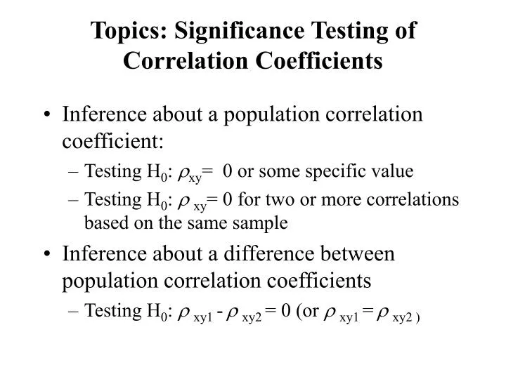
Topics: Significance Testing of Correlation Coefficients. Inference about a population correlation coefficient: Testing H 0 : xy = 0 or some specific value Testing H 0 : xy = 0 for two or more correlations based on the same sample

E N D
Topics: Significance Testing of Correlation Coefficients • Inference about a population correlation coefficient: • Testing H0: xy= 0 or some specific value • Testing H0: xy= 0 for two or more correlations based on the same sample • Inference about a difference between population correlation coefficients • Testing H0: xy1 -xy2 = 0 (or xy1 =xy2 )
Inference about a Correlation Coefficient • Purpose: to determine whether two variables (X and Y) are linearly related in the population. • H0: xy= 0 • H0: xy=some specified value
Test of Correlation Coefficient • H0: xy= some specified value • H1: xy not= some specified value ( < or > than some specified value) • Transform sample and population correlation coefficients to Zr and Z • Calculate t zobserved:distance of transformed rxy from the transformed population xy in standard error points • Test against zcritical (determined from table for chosen level of significance)
Example • Study of relationship between achievement motivation and performance in school (grade point average). Theory and prior research suggests that the correlation between these two variables is positive and moderately high (.50) • The observed correlation in this study was .75 based on N=63
Test of Correlation Coefficient: One Sample • H0: xy= .50 • H1: xy not= .50 • Level of Significance: .05 • Verify Assumptions • Independence of score pairs • Bivariate Normality • n >= 30
Assumptions • Independence: where the pair of scores for any particular student is independent of the pair of scores of every other student. • Bivariate Normality: For each value of X, the values of Y are normally distributed; for each value of Y the values of X are normally distributed; each variable normally distributed • Sample Size: n >= 30
Bivariate Normal For each value of X the Y scores are normally distributed For each value of Y the X scores are normally distributed
Example Con’td • Find Fisher Z transformation for rxy and xy (from a Table I) • r = .75 so Zr = .973 • = .50 so Z = .549 • Set up Zrobserved: Zr-Z/sZ to get distance of Zr from Z in standard error points • Computation formula for Zrobserved : • (Zr-Z) (sqrt n-3) = • (.973 - .549)/7.75 = • (.424)(7.75) = 3.29
Example Con’td • Find zcritical (from table or memory) = 1.96 • Decision Rule: • Reject H0 if absolute value of zrobserved >= 1.96 (3.29 is greater than 1.96) • Do not reject H0 if absolute value of zrobserved < 1.96 • Conclusion: the relationship between achievement motivation and school performance (grade point average) is greater than the specified value of .50
The Simple Approach When H0: xy= 0 • H0: xy= 0; H1: xy > 0 • Sample size = 102 • r = .24 • Compare robserved with r critical(.05,df=100) = .1638 (from Table G) • Since .24 > .1638 can reject the null hypothesis and conclude that there is a positive correlation in the population--our best estimate of that correlation is .24
Example: Testing Two or More Correlation Coefficients • Working example: Suppose the following measures were collected on 82 subjects: GPA,. Self-concept, and locus of control (internal-external)
Testing H0: xy= 0 for Two or More Correlations Based on Same Sample (N=82)
Testing H0: xy= 0 for Two or More Correlations Based on Same Sample • H0: • H1 (non-directional): • Level of significance: = .01 (level of significance) • Assumptions: • Number of Variables: • Number of dfs: • Critical Value (from Table H) • Decisions and conclusions:
Inference about Difference between Population Correlation Coefficients • To determine whether or not the observed difference between two correlation coefficients (r1-r2) may be due to chance or represents a difference in population coefficients
Example: Testing Difference between Two Correlation Coefficients • To determine whether or not the observed difference between two correlation coefficients (r1-r2) may be due to chance or represents a difference in population coefficients • In the Overachievement Study, the correlation between SAT scores and GPA was .0214 for the sample of 40 subjects. However the correlation between SAT and GPA for men was -.2369 and for women was +.3760.
Example: Differences (con’t) • H0: • H1 (non directional): • Significance Level: = .05 • Check assumptions • Convert sample r’s to Zrs (Table I): male Zrmale = -.239; female Zrfemale = .394 • Compute standard error of the difference between correlations: srmale-rfemale: .34 (via formula) • Calulate zrmale-rfemale(observed) = Zrmale- - Zrfemale/ srmale-rfemale : -.633/.34 = -1.86 • Find z rmale-rfemale(critical) : +/-1.96 (.05, two-tailed) • Decision and Conclusion: