Download

1 / 26
260 likes | 460 Views
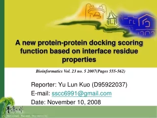
A new protein-protein docking scoring function based on interface residue properties. Reporter: Yu Lun Kuo (D95922037) E-mail: sscc6991@gmail.com Date: November 10, 2008. Bioinformatics Vol. 23 no. 5 2007(Pages 555-562). Introduction.

E N D
A new protein-protein docking scoring function based on interface residue properties Reporter: Yu Lun Kuo (D95922037) E-mail: sscc6991@gmail.com Date: November 10, 2008 Bioinformatics Vol. 23 no. 5 2007(Pages 555-562)
Introduction • A protein-protein docking procedure traditionally consist of two successive tasks • A search algorithm generates a large number of candidate solutions • Over the rotational/translational degrees of freedom • Two partners contact each other in many different orientations • A scoring function is used to rank them • The best solutions are selected by evaluating a score
Introduction • Scoring function • Express the geometric complementarity of the two molecular surfaces in contact • The strength of the interaction • Based on the physico-chemical characteristics of the amino acids in contact with each other
Introduction • The formation of a complex • Concern only the side chain conformation of amino acid residues at the interface • Imply motions of the protein backbone • The nature and amplitude of which remains very difficult to predict • Unbound docking predictions much more difficult than bound ones
Introduction • Protein-protein complexes in a complete genome with thousands of genes • Very reliable • The score of the best solution is high • The best solution is close to the native complex • Very fast • The inspection of a whole genome requires the modeling of many hundreds of thousands potential complexes
Methods • The Voronoi diagrams • Includes all points of space that are closer to the cell centroid than to any other centroid • Smallest polyhedron defined by bisecting planes between its centroid and all others • The Dalaunay tessellation is obtained by tracing the vertices joining centroids
Tessellation Definitions (1/2) • Two residues are neighbors • If their Voronoi cells share a common face • A residue belongs to the protein interior • If all its neighbors are residues of the same protein • A residue belongs to the protein surface • If one ore more of its neighbors is solvent
Tessellation Definitions (2/2) • A residue belongs to the protein–protein interface • If one or more of its neighbors belongs to the other protein • An interface residue belongs to the core of the interface • If none of its neighbors is solvent • The cell facets shared by residues of both proteins constitute the interface
Voronoi Description (1p2k) Protein chains Solvent By Voronoi polyhedra of residues of two proteins, representating the interface
Training Set • The training set consists in two subsets • Positive examples • Complexes of known 3D structure • The 2004 #1 of the Protein Data Bank (PDB) • Negative examples • Generated from the positive examples using a docking procedure • Decoys
Decoys • An imperfect scoring function can • Mislead by predicting incorrect ligand geometries by selecting nonbinding molecules over true ligands • These false-positive hits may be considered decoys
Training Attributes (1/2) • Number of parameters that may be used in • training is limited by the size of the training set • To define pair attributes, we grouped residue types in six categories • Hydrophobic H • Aromatic Φ • Positive charged + • Negatively charged – • Polar P • Small S
Training Attributes (2/2) • Attributes includes 84parameters in sixe classes • P1 The Voronoi interface area (1 parameter) • P2 Total number of core interface residues (1) • P3 Number fraction of each type of core interface residues (20) • P4 The meanvolume of the Voronoi cells for the core interface residues of each type (20) • P5 number fraction of pairs of each category (21) • P6 The mean centroid-centroid distance in pairs of each category (21)
Learning Methods • The values of the 84 parameters were measured on • The 102 native complexes (positive) • The decoys of training set (negative) • Logistic function • SVM (Support Vector Machines) • ROGER (a ROc based GEnetic learner)
Learning Methods • Logistic function • Linear combination of the parameters with weighted optimized to yield a value • Close to 1 on the native models • 0 on the decoys • Using the general linear model (GLM) of the R software
Learning Methods • SVM (Support Vector Machine) • Divide a high-dimensional space into regions containing only positive examples or only decoys • Using SVMTorch • Efficiently solve large-scale regression problems
Learning Methods • ROGER (Roc based genetic learner) • The receiver operating characteristics (ROC) procedure is often used evaluate learning • By cross-validation on examples • Uses genetic algorithm to find a family of functions that optimized the ROC criterion Central value ci and weight wi
Results and Discussion • Performance of the learning procedures • The ROC curve was evaluated on the training set for four different scores • Sum of the mean square deviation • Logistic function • SVMs • ROGER scoring function • A perfect selection (100% true positive &no false positive) should make the area under the ROC curve AUC equal to 1
ROGER and SVMs did much better • AUC of 0.98 and 0.99, respectively • Very few false positives among their best scoring solutions • Retained the ROGER score for further studies as the SVMs only give a binary classification • Ill-suited to our problem of “finding a needle in a hay stack”
Results on the targets of CAPRI rounds 3-6 • We tested the scoring functions on models of the targets of CAPRI rounds 3-6 • By two docking programs • DOCK (1991) • HADDOCK (2003)
Fnat: fraction of native contacts present in the solution • Fint: fraction of interface residues correctly predicted • Class 1: Fnat > 0.75 • Class 2: 0.5 < Fnat < 0.75 • Class 3: 0.25 < Fnat < 0.5 • Class4: 0 < Fnat < 0.25 • Class5: Fint > 0 and Fnat =0 • Class6: Fint = 0 and Fnat = 0
target The best rank given by our scoring function to a solution of the best class in the set Number of models with ROGER ranks < 50 that belong to the best class Original rank of the rank 1 solution Rank given by our function is better than given by HADDOCK Best class (class 2), re-ranked 4 Next best class (class 3) was1st Top 50 ROGER scores included 4 models of class 2, and 44 models of class 3 Thus Very few if any of top50 were false positive he first solution of the second best class (class 4 in this case) is ranked 1 target 18: the best solution in the set has 31% of native contacts. The best solution is the set is thus class 3.
Conclusion • For most targets, a best or second best class solution was found in the top 10 ranking solutions • More than half of the cases the top ranking solution belonged to the best or second best class • For all targets but one • Rank given to the first best class solution by our scoring function is better than the rank given by the original method (DOCK or HADDOCK)