Download
1 / 35
370 likes | 533 Views
Traffic flow on networks. Benedetto Piccoli Istituto per le Applicazioni del Calcolo “Mauro Picone” – CNR – Roma Joint work with G. Bretti, Y. Chitour, M. Garavello, R.Natalini , A. Sgalambro. Macroscopic models.

E N D
Traffic flow on networks Benedetto Piccoli Istituto per le Applicazioni del Calcolo “Mauro Picone” – CNR – Roma Joint work with G. Bretti, Y. Chitour, M. Garavello, R.Natalini , A. Sgalambro
Macroscopic models Vehicular traffic can be treated in different ways with microscopic,mesoscopic or macroscopic models. Macroscopic models mimic some phenomena such as the creation ofshocksand their propagation backwards along the road, since they candevelop discontinuities in a finite time even starting from smooth data. Representation of intersections: - Backward propagation of queues - Distribution of flow capacity resource on the downstream links of a node to its upstream links
Fluidodynamical models for traffic flow • LWR model M.J. Lighthill, G.B. Whitham, Richards 1955 • Example
Traffic features difficult to reproduce: traffic jams Empirical Evidences: • Once created, jams are stable and can move for hours against the flow of traffic • The flow out of a jam is a stable, reproducible quantity
Bilinear model • Simple model with reasonable properties • Two characteristic velocities • Respect phenomenon of backward moving clusters
Fluidodynamical models for traffic flow • Aw Rascle model Aw Rascle model solves typical problems of second order models: Cars going backwards! Other models: Greenberg, Helbing, Klar, Rascle, Benzoni - Colombo, etc.
Road networks • Road networds consists of a finite set of roads with junctions connecting roads : Problem: how to define a solution at junctions.
Solutions at junctions • Solve the Riemann problem at junctions • There are prescribed preference of drivers, i.e. traffic from incoming roads • distribute on outgoing roads according to fixed (probabilistic) coefficients (B) Respecting rule (A) drivers behave so as to maximize flow. • REMARK: • The only conservation of cars does not give uniqueness • Rule (A) implies conservation of cars • The only rule (A) does not give uniqueness
Rules (A) and (B) Rule (A) corresponds to fix a traffic distribution matrix Using rule (A) and (B) (under generic assumption on the matrix A), it is possible to define a unique solution to Riemann problems at junctions. Remark: other definition given by Holden-Risebro ’95.
LP problem at junctions It is enough to solve a LP problem at junctions for incoming fluxes! Then other fluxes and densities are determined. Other way of looking: Demand – Supply of J.P. Lebacque
Continuous dependence • Lipschitz continuous dependence does not hold: explicit counterexample. • Open problem: continuous dependence. • Lipschitz continuous dependence holds only for: • Single crossing with assumptions on initial data. • Small BV perturbations of generic equilibria. • Open problems: control the BV norm of density, extension to networks with any junction.
Numerical approximation • Approximation schemes (explicit schemes): • Godunov’s scheme (first order) • Kinetic scheme (kinetic scheme with 2 or 3 • velocities) of first order (Aregba-Driollet – Natalini) • Kinetic scheme with 3 velocities of second order • (Aregba-Driollet – Natalini)
Godunov scheme Construct piecewise constant approximation of the initial data : The scheme defines recursively starting from . CFL-like condition: The projection of the exact solution on a piecewise constant function is: These values are computed with the Gauss-Green formula.
Godunov’s scheme The scheme reads: with the numerical flux (associated to flux function ):
Kinetic scheme Drawback: • Diffusivity at first order for 2 velocities (Lax-Friedrichs scheme). Advantages of kinetic scheme: • Extension to High order • No instability at the boundary Godunov scheme: Kinetic scheme:
Large simulations • Necessity of simulating networks with thousands of arcs and nodes • Fast simulation to apply for optimization problems • Elaboration of big data bases for network characteristic • Visualization time
Modified Godunov IDEA: Use bilinear model to have simplified choices of Numerical fluxed
FVST scheme 1. Use simplified flux function with two characteristic speed 2. Make use of theoretical results to bound the number of regimes changes 3. Track exactly regimes changes or separating shocks and use simple dynamics for one-sided zones
FVST scheme Finite volumes shock tracking scheme: • Strongly bounded computational times • Error due only to initial data rounding and junction data rounding • Bounded to solutions for empty initial network
Networks and Heterogeneous Media
Packets flow on telecommunication networks Benedetto Piccoli Istituto per le Applicazioni del Calcolo “Mauro Picone” – CNR – Roma Joint work with C. D’Apice, R. Manzo, A. Marigo
Packets flow on telecommunication networks Telecommunication networks as Internet: no conservation of packets at small time scales. Assume there exists a loss probability function and packets are re-sent if lost. Then at 1st step: (1-p) packets sent, p lost at 2nd step: p(1-p) packets sent, p^2 lost …. at kth step: p^(k-1) (1-p) sent, p^k lost … Finally the average transmission time and velocity are:
Riemann problems at junctions Maximize the fluxes over incoming and outgoing lines: remove rule (A)
BV Estimates For interactions with a junction we get: For special flux fuction we get BV estimates on the densities.