Download
1 / 32
320 likes | 481 Views
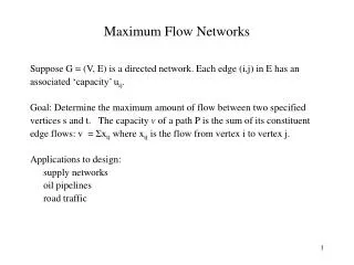
Maximum Flow Networks. Suppose G = (V, E) is a directed network. Each edge (i,j) in E has an associated ‘capacity’ u ij . Goal: Determine the maximum amount of flow between two specified vertices s and t. The capacity v of a path P is the sum of its constituent

E N D
Maximum Flow Networks Suppose G = (V, E) is a directed network. Each edge (i,j) in E has an associated ‘capacity’ uij. Goal: Determine the maximum amount of flow between two specified vertices s and t. The capacity v of a path P is the sum of its constituent edge flows: v = Σxij where xij is the flow from vertex i to vertex j. Applications to design: supply networks oil pipelines road traffic
Background Assumptions: • Integer data • Directed network • Nonnegative capacities on each arc • Vertex s is the source • Vertex t is the sink Definitions: • Residual network • Cut Techniques: • Augmenting Paths – Examine residual network for s-t paths. • Preflow-Push – Flow moved according to individual edge not path.
Maximum Flow as Linear Programming Problem subject to
Example 2,4 2 4 4,7 3,9 1,2 2,6 s t 8,8 7,9 3 Each edge is labeled as (xij, uij) = (flow, capacity). However, this flow value, v(x) = 11, is not a maximum.
Residual Network Given a current flow x, keep track of how much further the flow can be increased in each direction of the edge. xij, uij For any edge in G: i j uij -xij The corresponding edge (with capacities) in residual network of G: i j xij The residual network of G, G(x), has edges with positive residual capacity, rij = uij – xij + xji. In general, it is the amount by which we can further increase flow from i to j in the current network.
2,4 2 4 4,7 3,9 1,2 2,6 s t 8,8 7,9 3 Example – Re-examined 2 3 2 4 3 2 1 2 6 4 s t 1 6 2 8 7 3 Network with flows and capacities. Residual network with capacities. We know this network flow is not a maximum. How can we get a better one? What do we do in general?
Cuts A cut is defined by a partition of the vertex set E into subsets S and S* = E – S. The cut [S,S*] consists of all edges with one endpoint in S and the other in S*. The forward edges of [S,S*] are denoted (S, S*). The backward edges are denoted as (S*,S). An s-t cut [S,S*] has s in S and t in S*. The removal of the forward edges in an s-t cut will separate vertices s and t. That is, there is no longer a directed s to t path. The capacity of any cut [S,S*], u[S,S*], is the sum of the capacities of the forward edges of the cut. u[S,S*] is an upper bound on the amount of flow sent from S to S*. A minimum s-t cut has the smallest capacity among all s-t cuts.
Examples of 1-6 cuts 5 5 2 4 2 4 8 8 10 10 1 4 6 4 1 6 8 8 8 8 10 10 3 3 5 5 5 5 S = { } S* = { } Forward edges of [S,S*]= { } u[S, S*] = = S = { } S* = { } Forward edges of [S,S*]= { } u[S, S*] = =
Theorems Theorem If x is any feasible flow and if [S,S*] is any s-t cut, then the flow value, v(x), from s to t is at most u[S,S*]. Corollary the max flow value ≤ the minimum cut capacity Max-Flow Min-Cut Theorem For any capacitated network, the value of the maximum s-t flow, x’, equals the capacity of a minimum s-t cut, [S,S*]. v(x’) = u [S,S*]
Improving a Flow • Given the flow x, look for a path P from s to t in the residual network G(x) along which flow can be sent. Then send as much flow along P as possible. • We call any directed path P from s to t in the residual network an augmenting path. The residual capacity of such a path is δ(P) = min{rij:(i, j) P). • To augment along P is to send δ(P) units of flow along each edge of the path. We then modify x and the residual capacities rij appropriately. • rij := rij – δ(P) for each edge (i,j) P • rji := rji + δ(P) for each edge (i, j) P • Result: flow value, v, increases by δ(P).
4,4 2,4 2 2 4 4 4,7 6,7 5,9 3,9 1,2 1,2 2,6 2,6 s s t t 8,8 8,8 7,9 7,9 3 3 Example 2 3 2 4 3 2 1 2 6 4 s t 1 6 2 8 7 3 Network with flows and capacities. v =11 Residual network with capacities. Augment along path P = s-2-4-t. δ(P) = min{6, 2, 3} = 2. new flow value =13 5 2 4 1 4 1 2 4 6 s t 1 6 2 8 7 3
Example – Augmenting Paths Step 0: initial residual graph is original 4 4 4 4 2 4 2 4 6 2 8 4 1 2 3 6 1 2 3 6 2 5 2 8 5 3 5 1 3 5 3 5 6 5 Step 3: Push 2 units along path 1-2-5-4-6 Step 1: Push 4 units along path 1-2-4-6 4 4 4 2 4 4 6 2 2 4 6 4 1 2 3 6 2 2 1 2 1 6 2 8 5 5 2 3 5 3 5 1 3 5 6 5 Step 2: Push 5 units along path 1-3-5-6 Step 4: Push 1 units along path 1-3-5-4-6
Example – continued 4 7 2 4 6 1 1 2 3 6 4 6 2 2 5 2 4 6 3 5 6 8 1 2 3 6 No more augmenting paths 2 8 5 3 5 6 4,4 2 4 7,8 6,6 1 0,2 3,3 6 2,2 6,8 5,5 3 5 6,6 Maximum Flow in G is 12
THEOREM The following are equivalent statements • The s-t flow x’ with value v(x’) is maximum • G(x’) contains no augmenting path. • There is an s-t cut [S,S*] with u[S,S*] = v(x’)
Generic Augmenting Path Algorithm • In this algorithm, we keep sending flow along augmenting paths until no s-t path exists in the residual network. • Can carry out calculations entirely on G(x). • Flows in G are found at the very end. algorithmaugmenting_path; begin x := 0 while G(x) contains a directed path from s to t do begin P = Find_Path(s, t, G(x)); δ(P) := min{rij: (i,j) P}; augment δ(P) units of flow along P; update G(x); end; end;
Find_Path Options • More than one way to pick an augmenting path • “Poor” choices can lead to many augmentations. • Info lost when successive paths are found. • Balance effort to find a “good” path with the reduction in # of augmentations. • Maximum capacity – select path P such that δ(P) is as large as possible. • Shortest path – use the path with the minimum number of edges. • Scaling – successively solve subproblems with a certain capacity. 3 50 50 1 1 4 50 50 2
Distance Labels • For the “shortest path” version of the augmenting path algorithm and for another max flow algorithm, the pre-flow push, the notion of distance labels is needed. • The distance label d(j) is a nonnegative integer assigned to each j in G(x). • The distance labels are valid if d(t) = 0 d(i) ≤ d(j)+1 for each (i,j) G(x) • If d(j) are valid, then d(j) is a lower bound on the shortest distance from j to t. • If d(s) ≥ n then there is no s-t path in G(x). (n = number of vertices in G) • An admissible edge in G(x) is one where d(i) = d(j) + 1. • An admissible path is a path from s to t consisting of admissible edges and is a shortest augmenting path from s to t. 3 4 1 5 2
Shortest Distance Algorithm • Admissible paths are successively built by advancing until vertex t is reached. • If no admissible edge is available at some point, then retreat and relabel will be a way of updating distances in the new residual graph. • In this way, we maintain valid distance labels without starting from scratch. algorithmshortest augmenting path; begin x:= 0; calculate exact distance labels, d(j) to vertex t; j := s; while d(s) <n do begin if j has an admissible edge then begin advance(j); if j = t then augment and set j := s; end; elseretreat(j); end; end;
algorithmadvance(j); begin let (j,k) be an admissible edge from j; pred(k)=j; j := k; end; algorithmretreat(j); begin d(j) := min{d(k)+1: (j,k) in E(j) with rjk > 0}; if E(j) with rjk > 0 empty then d(j) = n; if j ≠ s then j := pred(k); end; algorithmaugment; begin derive path P from pred; δ(P) := min{rij: (i,j) P}; augment δ(P) units of flow along P; end;
Example d(3)=1 3 3 5 5 4 4 d(1)=2 d(4)=0 3 3 1 4 1 4 2 1 1 1 1 2 2 d(2)=1 1. Calculate d(j) 3. Advance 1-2, retreat, relabel vertex 2 d(3)=1 d(3)=1 3 3 5 5 4 4 d(1)=2 d(1)=2 d(4)=0 d(4)=0 3 3 1 4 1 4 2 1 1 1 1 2 2 d(2)=1 d(2)=2 4. Advance 1-3-4, δ(P) =4, augment 2. Advance 1-2-4, δ(P) =1, augment
Example d(3)=1 d(3)=1 3 3 4 5 4 4 d(1)=2 d(1)=3 1 d(4)=0 d(4)=0 3 2 1 1 4 1 4 1 1 1 2 1 2 2 d(2)=2 d(2)=2 7. Advance 1, retreat, relabel 1 5. Advance 1, retreat relabel 1 d(3)=1 d(3)=1 3 5 3 4 4 4 d(1)=4 d(4)=0 d(1)=3 1 d(4)=0 2 1 1 4 3 1 4 1 2 1 1 1 2 2 d(2)=2 d(2)=2 6. Advance 1-2-3-4, δ(P) =1, augment 8. Maximum Flow achieved
Example - Results 3 5,5 4,4 Note monotonicity of distance labels 1,3 1 4 2,2 1,1 2 Note monotonicity of path lengths 1-2-4 1-3-4 1-2-3-4
Additional Exercises 18 3 6 22 25 17 30 19 sink 11 21 1 4 5 8 13 source 17 24 26 22 2 7 4 7 3 6 3 5 8 11 6 9 3 1 1 source 2 4 10 11 1 1 4 7 1 6 2 source 9 5 1 7 7 sink 3 2 5 2 6 sink 8 2
Preflow-push Algorithm • Distance labels – d(t) = 0; d(i) ≤d(j) + 1 for each (i,j) in G(x) • Excess flow – e(i) = excess at each vertex for a given preflow • Active vertices – vertices with positive excess • Admissible edges – edges that satisfy the condition that d(i) = d(j) + 1 • Preflow – infeasible solution; • Algorithm strives for feasibility/optimality when all excess at sink and source algorithmpreflow-push; begin preprocess; while network contains an active vertex do begin select an active node i; push/relabel(i); end; end;
algorithmpreprocess; begin x := 0; compute the exact distance labels d(i) from s; xsj := usj for each edge (s,j) in E(s); d(s) := n end; algorithmpush/relabel(i); begin if the networks contains an admissible edge (i,j) then push δ = min{e(i), rij} units of flow from vertex i to vertex j; else replace d(i) by min{d(j)+1: (i,j) in E(i) and rij > 0}; end;
Example 1. Network G 2. preprocess: first residual graph Active nodes: 2, 3 Active nodes: e(3)=0 d(3)=1 e(3)=4 d(3)=1 3 3 5 5 e(1)=0 d(1)=2 4 e(1)=0 d(1)=4 4 3 e(4)=0 d(4)=0 3 e(4)=0 d(4)=0 1 4 1 4 2 1 2 1 2 2 e(2)=0 d(2)=1 e(2)=2 d(2)=1
Example Selected node: 2 Selected node: 3 Active nodes: 3 Active nodes: 2 3. Saturating push of 1 unit along 2-4; Relabel distance node 2 4. Push of 4 units along 3-4 Active nodes: 3, 2 Active nodes: 2 e(3)=4 d(3)=1 e(3)=0 d(3)=1 3 3 5 1 e(1)=0 d(1)=4 4 e(1)=0 d(1)=4 4 4 3 e(4)=1 d(4)=0 3 e(4)=5 d(4)=0 1 4 1 4 2 1 2 1 2 2 e(2)=1 d(2)=2 e(2)=1 d(2)=2
Example Selected node: 2 Selected node: 3 Active nodes: Active nodes: 5. Push of 1 unit along 2-3 6. Saturating Push of 1 units along 3-4 Active nodes: 3 Active nodes: e(3)=1 d(3)=1 e(3)=0 d(3)=1 3 3 1 e(1)=0 d(1)=4 4 e(1)=0 d(1)=4 4 4 5 2 e(4)=5 d(4)=0 1 1 4 2 1 e(4)=6 d(4)=0 1 4 2 1 2 1 2 2 e(2)=0 d(2)=2 e(2)=0 d(2)=2
Preflow-Push: Example 2 5 2 4 8 10 6 1 8 8 10 3 5 5
Checking if feasible flow exists • Let G = (V,E) be a network with supplies and demands at each vertex • b(j) > 0 indicates supply at vertex j • b(j)<0 indicates demand at vertex j • Assumption: Σb(j) = 0 • Does a flow, x, exist? • Transform into a maximum flow network, G’ • Add a source vertex, s, and a sink vertex, t. • Add edge (s, j) with capacity, rsj=b(j), if b(j)>0 • Add edge (j, t) with capacity, rjt=b(j), if b(j)<0 • Solve max flow from s to t • Result: If the max flow in G’ saturates all the source and sink edges, then the original problem has a feasible solution. Otherwise, infeasible.
Example 1-Feasible Flow? b(2) = 5 2 b(1) = 4 4 6 4 4 b(4) = -7 1 2 8 3 b(3) = -2
Example 2-Feasible flow? b(2) = 5 2 b(1) = 4 4 6 1 4 b(4) = -7 1 3 8 3 b(3) = -2