Download
1 / 38
420 likes | 616 Views
Learn about graphical, bisectional, and false-position methods to find roots of equations in this comprehensive chapter. Understand the principles of root-finding and apply these techniques in engineering problems effectively.

E N D
Bracketing Methods Chapter 5 Lecture Notes Dr. Rakhmad Arief Siregar Universiti Malaysia Perlis Applied Numerical Method for Engineers
Roots of equations • Roots of equation represent the value of x that make that equation equal to zero. • Years ago, you learned to use the quadratic formula: • to solve
Graphical Methods • The simple method for obtaining an estimate of the root of the equation f(x)=0 is to make a plot of the function and observe where it crosses the x axis. • This point, provide a rough approximation of the root
Ex. 5.1 Graphical Approach • Use the graphical approach to determine the drag coefficient, c, needed for a parachutist of mass m = 68.1 kg to have a velocity of 40 m/s after free-falling for time t = 10 s. The acceleration due to gravity is 9.8 m/s2 • Solution • By inserting t=10, g=9.8, v=40 and m =68.1
Ex. 5.1 Graphical Approach • The root is between 12 and 16. • By visual inspection, the point is roughly at 14.75 • Lets checks the point by substituting into equation • which is close to zero. • Lets check the velocity
Illustration of number of general ways Same sign of bounds Opposite sign of bounds No root or an even number of root An odd number of root
Same Exception • Multiple root that occurs when the function is tangential to x axis • Discontinuous function where end points of opposite sign bracket an even number of roots
f(x) = sin 10x + cos 3x • The previous figure showed that f(x) changed sign on opposite sides of the root • In general, if f(x) is real and continuous in the interval from xl to xu and f(xl) and f(xu) have opposite signs that is • Then there is at least one real root between xl to xu
The Bisectional Method • The bisectional method, which is alternatively called binary chopping, interval halving, or Bolzano’s method. • If a function changes sign over an interval is always divided in half. • The location of the root is then determined as lying at the midpoint of the subinterval within which the sign change occurs • The process is repeated to obtain refined estimates
Ex. 5.3 Bisection • Use bisectional to solve the same problem approached graphically in Ex. 5.1
Ex. 5.3 Bisection • Step 1 Choose lower and upper bound, say 12 and 16. the initial estimate of the root xr , lies at the midpoint of the interval • Check or • f(12)f(14)= 6.067(1.569)=9.517 upper subinterval • the root must be located between 14 and 16
Ex. 5.3 Bisection • Step 2 Choose lower and upper bound, say 14 and 16. the initial estimate of the root xr , lies at the midpoint of the interval • Check • f(14)f(15)= 1.569(-0.425)=-0.666 lower subinterval • the root must be located between 14 and 15
Ex. 5.3 Bisection • Step 3 Choose lower and upper bound, say 14 and 15. the initial estimate of the root xr , lies at the midpoint of the interval • Check • f(14)f(14.5)= 1.569(0.552)=0.866088 upper subinterval • the root must be located between 14.5 and 15
Ex. 5.3 Bisection • Step 4, 5, etc • Follow the procedures finally you will yields the true value of the root is 14.7802
Termination criteria and • Error estimates
Problem 5. 1 • Graphical solution
The False-Position Method • Although bisection is a perfectly valid technique for determining roots, its “brute-force” approach is relatively inefficient. • False position is an alternative based on a graphical insight. • In latin, it is called as regula falsi • Other name of this method is the Linear Interpolation Method
Ex. 5.5 False Position Method • Use the false-position method to determine the root of the same equation investigated in Ex. 5.1
Ex. 5.5 False Position Method • As in Ex. 5.3, initial the computation with guesses of xl = 12 and xu = 16 • First step: • xl = 12 f(12) = 6.0699 • xu = 16 f(16) = -2.2688 • Check Lower subinterval
Ex. 5.5 False Position Method • Second step, set xl = 12 and xu = 14.9113: • xl = 12 f(12) = 6.0699 • xu = 14.9113 f(14.9113) = -0.2543 • Check
Comparison • Which one is more efficient?
Pitfalls of the False-Position Method • Although the false-position method would seem much more superior compare to the bracketing method, there is cases where it performs poorly • In fact, in certain cases, bisection yields superior results
Ex. 5.6 Where bisection is preferable to false position • Use bisection and false position to locate the root of f(x) = x10 – 1between x = 0 and x = 1.3